Model Management Guidance
Definitions and Interpretations
The following terms shall have the meaning assigned to them for the purpose of interpreting these Standards and the related Guidance:
1. Board: As defined in the CBUAE’s Corporate Governance Regulation for Banks.
2.Causality:
(written in lower case as “causality”): Relationship between cause and effect. It is the influence of one event on the occurrence of another event.
3.CBUAE: Central Bank of the United Arab Emirates.
4.Correlation
(written in lower case as “correlation”): Any statistical relationship between two variables, without explicit causality explaining the observed joint behaviours. Several metrics exist to capture this relationship. Amongst others, linear correlations are often captured by the Pearson coefficient. Linear or non-linear correlation are often captured by the Spearman’s rank correlation coefficient.
5.Correlation Analysis:
(written in lower case as “correlation analysis”): Correlation analysis refers to a process by which the relationships between variables are explored. For a given set of data and variables, observe (i) the statistical properties of each variable independently, (ii) the relationship between the dependent variable and each of the independent variables on a bilateral basis, and (iii) the relationship between the independent variables with each other.
6.CI:
(Credit Index): In the context of credit modelling, a credit index is a quantity defined over (-∞,+∞) derived from observable default rates, for instance through probit transformation. CI represents a systemic driver of creditworthiness. While this index is synthetic, (an abstract driver), it is often assimilated to the creditworthiness of specific industry or geography.
7.Default:
(written in lower case as “default”): The definition of default depends on the modelling context, either for the development of rating models or for the calibration and probabilities of default. For a comprehensive definition, refer to the section on rating models in the MMG.
8.Deterministic Model:
(written in lower case as “deterministic model”): A deterministic model is a mathematical construction linking, with certainty, one or several dependent variables, to one or several independent variables. Deterministic models are different from statistical models. The concept of confidence interval does not apply to deterministic models. Examples of deterministic models include NPV models, financial cash flow models or exposure models for amortizing facilities.
9.DMF:
(Data Management Framework): Set of policies, procedures and systems designed to organise and structure the management of data employed for modelling.
10.DPD:
(Days-Past-Due): A payment is considered past due if it has not been made by its contractual due date. The days-past-due is the number of days that a payment is past its due date, i.e. the number of days for which a payment is late.
11.DSIB:
(Domestic Systemically Important Banks): These are UAE banks deemed sufficiently large and interconnected to warrant the application of additional regulatory requirements. The identification of the institutions is based upon a framework defined by the CBUAE.
12.EAD:
(Exposure At Default): Expected exposure of an institution towards an obligor (or a facility) upon a future default of this obligor (or its facility). It also refers to the observed exposure upon the realised default of an obligor (or a facility). This amount materialises at the default date and can be uncertain at reporting dates prior to the default date. The uncertainty surrounding EAD depends on the type of exposure and the possibility of future drawings. In the case of a lending facility with a pre-agreed amortisation schedule, the EAD is known. In the case of off-balance sheet exposures such as credit cards, guarantees, working capital facilities or derivatives, the EAD is not certain on the date of measurement and should be estimated with statistical models.
13.EAR: (Earning At Risk): Refer to NII.
14.ECL:
(Expected Credit Loss): Metric supporting the estimation of provisions under IFRS9 to cover credit risk arising from facilities and bonds in the banking book. It is designed as a probability-weighted expected loss.
15.Economic Intuition:
(written in lower case as “economic intuition”): Also referred to as economic intuition and business sense. Property of a model and its output to be interpreted in terms and metrics that are commonly employed for business and risk decisions. It also refers to the property of the model variables and the model outputs to meet the intuition of experts and practitioners, in such a way that the model can be explained and used to support decision-making.
16.Effective Challenge:
Characteristic of a validation process. An effective model validation ensures that model defects are suitably identified, discussed and addressed in a timely fashion. Effectiveness is achieved via certain key features of the validation process such as independence, expertise, clear reporting and prompt action from the development team.
17. EVE :
(Economic Value of Equity): It is defined as the difference between the present value of the institution’s assets minus the present value of liabilities. The EVE is sensitive to changes in interest rates. It is used in the measurement of interest rate risk in the banking book.
18.Expert-Based Models:
(written in lower case as “expert-based models”): Also referred to as judgmental models, these models rely on the subjective judgement of expert individuals rather than on quantitative data. In particular, this type of model is used to issue subjective scores in order to rank corporate clients.
19.Institutions:
(written in lower case as “institution(s)”): All banks licensed by the CBUAE. Entities that take deposits from individuals and/or corporations, while simultaneously issuing loans or capital market securities.
20.LGD :
(Loss Given Default): Estimation of the potential loss incurred by a lending institution upon the default of an obligor (or a facility), measured as a percentage of the EAD. It also refers to the actual loss incurred upon past defaults also expressed as a percentage of EAD. The observed LGD levels tend to be related to PD levels with various strength of correlation.
21.Limits and limitations:
(written in lower case as “limits” and “limitations”): Model limits are thresholds applied to a model’s outputs and/or its parameters in order to control its performance. Model limitations are boundary conditions beyond which the model ceases to be accurate.
22.LSI :
(Large and/or Sophisticated Institutions): This group comprises DSIBs and any other institutions that are deemed large and/or with mature processes and skills. This categorisation is defined dynamically based on the outcome of regular banking supervision.
23.Macroeconomic Model:
(written in lower case as “macroeconomic model” or “macro model”): Refers to two types of models. (i) A model that links a set of independent macro variables to another single dependent macro variable or to several other dependent macro variables or (ii) a model that links a set of independent macro variables to a risk metric (or a set of risk metrics) such as probabilities of default or any other business metric such as revenues.
24.Market Data:
Refers to the various data attributes of a traded financial instrument reported by a trading exchange. It includes the quoted value of the instrument and/or the quoted parameters of that instrument that allow the derivation of its value. It also includes transaction information including the volume exchanged and the bid-ask spread.
25.Materiality:
The materiality of a model represents the financial scope covered by the model in the context of a given institution. It can be used to estimate the potential loss arising from model uncertainty (see Model Risk). Model materiality can be captured by various metrics depending on model types. Typically, total exposure can be used as a metric for credit models.
26.MMG: CBUAE’s Model Management Guidance.
27.MMS: CBUAE’s Model Management Standards.
28.Model:
(written in lower case as “model”): A quantitative method, system, or approach that applies statistical, economic, financial, or mathematical theories, techniques, and assumptions to process input data into quantitative estimates. For the purpose of the MMS and MSG, models are categorised in to three distinct groups: statistical models, deterministic models and expert-based models.
29.Model Calibration:
(written in lower case as “model calibration”): Key step of the model development process. Model calibration means changing the values of the parameters and/or the weights of a model, without changing the structure of the model, i.e. without changing the nature of the variables and their transformations.
30.Model Complexity:
(written in lower case as “model complexity”): Overall characteristic of a model reflecting the degree of ease (versus difficulty) with which one can understand the model conceptual framework, its practical design, calibration and usage. Amongst other things, such complexity is driven by, the number of inputs, the interactions between variables, the dependency with other models, the model mathematical concepts and their implementation.
31.Model Construction:
(written in lower case as “model construction”): Key step of the model development process. The construction of a model depends on its nature, i.e. statistical or deterministic. For the purpose of the MMS and the MMG, model construction means the following: for statistical models, for a given methodology and a set of data and transformed variables, it means estimating and choosing, with a degree of confidence, the number and nature of the dependent variables along with their associated weights or coefficients. For deterministic models, for a given methodology, it means establishing the relationship between a set of input variables and an output variable, without statistical confidence intervals.
32.Model Development: (written in lower case as “model development”): Means creating a model by making a set of sequential and recursive decisions according to the steps outlined in the dedicated sections of the MMS. Model re-development means conducting the model development steps again with the intention to replace an existing model. The replacement may, or may not, occur upon re-development.
33.Modelling Decision:
(written in lower case as “modelling decision”): A modelling decision is a deliberate choice that determines the core functionality and output of a model. Modelling decisions relate to each of the steps of the data acquisition, the development and the implementation phase. In particular, modelling decisions relate to (i) the choice of data, (ii) the analysis of data and sampling techniques, (iii) the methodology, (iv) the calibration and (v) the implementation of models. Some modelling decisions are more material than others. Key modelling decisions refer to decisions with strategic implications and/or with material consequences on the model outputs.
34.Model Risk:
Potential loss faced by institutions from making decisions based on inaccurate or erroneous outputs of models due to errors in the development, the implementation or the inappropriate usage of such models. Losses incurred from Model Risk should be understood in the broad sense as Model Risk has multiple sources. This definition includes direct quantifiable financial loss but also any adverse consequences on the ability of the institution to conduct its activities as originally intended, such as reputational damage, opportunity costs or underestimation of capital. In the context of the MMS and the MMG, Model Risk for a given model should be regarded as the combination of its materiality and the uncertainty surrounding its results.
35.Model Selection:
(written in lower case as “model selection”): This step is part of the development process. This means choosing a specific model amongst a pool of available models, each with a different set of variables and parameters.
36.Model Uncertainty:
(written in lower case as “model uncertainty”): This refers to the uncertainty surrounding the results generated by a model. Such uncertainty can be quantified as a confidence interval around the model output values. It is used as a component to estimate Model Risk.
37.Multivariate Analysis:
(written in lower case as “multivariate analysis”): For a given set of data and variables, this is a process of observing the joint distribution of the dependent and independent variables together and drawing conclusions regarding their degree of correlation and causality.
38.NII:
(Net Interest Income): To simplify notations, both Net Interest Income (for conventional products) and/or Net Profit Income (for Islamic Products) are referred to as “NII”. In this context, ‘profit’ is assimilated as interest. It is defined as the difference between total interest income and total interest expense, over a specific time horizon and taking into account hedging. The change in NII (“∆NII”) is defined as the difference between the NII estimated with stressed interest rates under various scenarios, minus the NII estimated with the interest rates as of the portfolio reporting date. ∆NII is also referred to as earnings at risk (“EAR”).
39.NPV :
(Net Present Value): Present value of future cash flows minus the initial investment, i.e. the amount that a rational investor is willing to pay today in exchange for receiving these cash flows in the future. NPV is estimated through a discounting method. It is commonly used to estimate various metrics for the purpose of financial accounting, risk management and business decisions.
40.PD:
(Probability of Default): Probability that an obligor fails to meet its contractual obligation under the terms of an agreed financing contract. Such probability is computed over a given horizon, typically 12 months, in which case it is referred to as a 1-year PD. It can also be computed over longer horizons. This probability can also be defined at several levels of granularity, including, but not limited to, single facility, pool of facilities, obligor, or consolidated group level.
41.PD Model:
(written as “PD model”): This terminology refers to a wide variety of models with several objectives. Amongst other things, these models include mapping methods from scores generated by rating models onto probability of defaults. They also include models employed to estimate the PD or the PD term structure of facilities, clients or pool of clients.
42.PD Term Structure:
(written as “PD term structure”): Refers to the probability of default over several time horizons, for instance 2 years, 5 years or 10 years. A distinction is made between the cumulative PD and the marginal PD. The cumulative PD is the total probability of default of the obligor over a given horizon. The marginal PD is the probability of default between two dates in the future, provided that the obligor has survived until the first date.
43.PIT (Point-In-Time) and TTC (Through-The-Cycle):
A point-in-time assessment refers to the value of a metric (typically PD or LGD) that incorporates the current economic conditions. This contrasts with a through-the-cycle assessment that refers to the value of the same metric across a period covering one or several economic cycles.
44.Qualitative validation:
A review of model conceptual soundness, design, documentation, and development and implementation process.
45.Quantitative validation:
A review of model numerical output, covering at least its accuracy, degree of conservatism, stability, robustness and sensitivity.
46.Rating/Scoring:
(written in lower case “rating or scoring”): For the purpose of the MMS and the MMG, a rating and a score are considered as the same concept, i.e. an ordinal quantity representing the relative creditworthiness of an obligor (or a facility) on a predefined scale. ‘Ratings’ are commonly used in the context of corporate assessments whilst ‘scores’ are used for retail client assessments.
47.Restructuring:
(written in lower case “restructuring”): The definition of restructuring / rescheduling used for modelling in the context of the MMS and MMG should be understood as the definition provided in the dedicated CBUAE regulation and, in particular, in the Circular 28/2010 on the classification of loans, with subsequent amendments to this Circular and any new CBUAE regulation on this topic.
48.Rating Model:
(written in lower case “rating model”): The objective of such model is to discriminate ex-ante between performing clients and potentially non-performing clients. Such models generally produce a score along an arbitrary scale reflecting client creditworthiness. This score can subsequently mapped to a probability of default. However, rating models should not be confused with PD models.
49.Retail Clients:
(written in lower case as “retail clients”): Retail clients refer to individuals to whom credit facilities are granted for the following purpose: personal consumer credit facilities, auto credit facilities, overdraft and credit cards, refinanced government housing credit facilities, other housing credit facilities, credit facilities against shares to individuals. It also includes small business credit facilities for which the credit risk is managed using similar methods as applied for personal credit facilities.
50.Segment:
(written in lower case as “segment”): Subsets of an institution’s portfolio obtained by splitting the portfolio by the most relevant dimensions which explain its risk profile. Typical dimensions include obligor size, industries, geographies, ratings, product types, tenor and currency of exposure. Segmentation choices are key drivers of modelling accuracy and robustness.
51.Senior Management: As defined in the CBUAE’s Corporate Governance Regulation for Banks.
52.Statistical Model:
(written in lower case as “statistical model”): A statistical model is a mathematical construction achieved by the application of statistical techniques to samples of data. The model links one or several dependent variables to one or several independent variables. The objective of such a model is to predict, with a confidence interval, the values of the dependent variables given certain values of the independent variables. Examples of statistical models include rating models or value-at-risk (VaR) models. Statistical models are different from deterministic models. By construction, statistical models always include a degree of Model Risk.
53.Tiers: Models are allocated to different groups, or Tiers, depending on their associated Model Risk.
54.Time series analysis:
(written in lower case as “time series analysis”): For a given set of data and variables, this is a process of observing the behaviour of these variables through time. This can be done by considering each variable individually or by considering the joint pattern of the variables together.
55.UAT:
(User Acceptance Testing): Phase of the implementation process during which users rigorously test the functionalities, robustness, accuracy and reliability of a system containing a new model before releasing it into production.
56.Variable Transformation:
(written in lower case as “variable transformation”): Step of the modelling process involving a transformation of the model inputs before developing a model. Amongst others, common transformations include (i) relative or absolute differencing between variables, (ii) logarithmic scaling, (iii) relative or absolute time change, (iv) ranking, (v) lagging, and (vi) logistic or probit transformation.
57.Wholesale Clients:
(written in lower case as “wholesale clients”): Wholesale clients refer to any client that is not considered as a retail client as per the definition of these Standards.
1 Context and Objective
1.1 Regulatory Context
1.1.1
The Risk Management Regulation (Circular No. 153/2018) issued by the Central Bank of the UAE (“CBUAE”) on 27th May 2018 states that banks must have robust systems and tools to assess and measure risks.
1.1.2
To set out modelling requirements for licensed banks, the CBUAE has issued Model Management Standards (“MMS”) and Model Management Guidance (“MMG”). Both MMS and MMG should be read jointly as they constitute a consistent set of requirements and guidance, as follows:
(i)
The MMS outline general standards applicable to all models and constitute minimum requirements that must be met by UAE banks.
(ii)
The MMG expands on technical aspects that are expected to be implemented by UAE banks for certain types of models. Given the wide range of models and the complexity of some, the CBUAE recognises that alternative approaches can be envisaged on specific technical points. Whilst this MMG neither constitutes additional legislation or regulation nor replaces or supersedes any legal or regulatory requirements or statutory obligations, deviations from the MMG should be clearly justified and will be subject to CBUAE supervisory review.
1.2 Objectives
1.2.1
Both the MMS and MMG share three key objectives. The first objective is to ensure that models employed by UAE banks meet quality standards to adequately support decision-making and reduce Model Risk. The second objective is to improve the homogeneity of model management across UAE banks. The third objective is to mitigate the risk of potential underestimation of provisions and capital across UAE banks.
1.2.2
The MMG outlines techniques based on commonly accepted practices by practitioners and academics, internationally. The majority of its content has been subject to consultation with numerous subject matter experts in the UAE and therefore it also reflects expected practices amongst UAE institutions.
1.3 Document Structure
1.3.1
Each section of the MMG addresses a different type of model. The MMG is constructed in such a way that the numbering of each article is sequentially and each article is a unique reference across the entire MMG.
1.3.2
Both the MMS and the MMG contain an appendix summarising the main numerical limits included throughout each document respectively. Such summary is expected to ease the implementation and monitoring of these limits by both institution and the CBUAE.
1.4 Scope of Application
1.4.1
The MMG applies to all licensed banks in the UAE, which are referred to herein as “institutions”.
1.4.2
The scope of institutions is consistent across the MMS and the MMG. Details about the scope of institutions are available in the MMS.
1.4.3
Branches or subsidiaries of foreign institutions should apply the most conservative practices between the MMG and the expectations from their parent company’s regulator.
1.4.4
Institutions with a parent company incorporated in the UAE should ensure that all their branches and subsidiaries comply with the MMG.
1.5 Requirements and Timeframe
1.6 Scope of Models
1.6.1
The MMG focuses on the main credit risk models entering the computation of the Expected Credit Loss in the context of the current accounting requirements, due to their materiality and their relevance across the vast majority of institutions. The MMG also provides guidance on other models used for the assessment of interest rate risk in the banking book and net present values.
1.6.2
The MMG does not impose the use of these models. The MMG outlines minimum expected practices if institutions decide to use such models, in order to manage Model Risk appropriately.
1.6.3
As model management matures across UAE institutions, additional model types may be included in the scope of the MMG in subsequent publications.
Table 1: List of model types covered in the MMG
Model type covered in the MMG Rating Models PD Models LGD Models Macro Models Interest Rate Risk In the Banking Book Models Net Present Value Models 2 Rating Models
2.1 Scope
2.1.1
The vast majority of institutions employ rating models to assess the credit worthiness of their obligors. Rating models provide essential metrics used as foundations to multiple core processes within institutions. Ratings have implications for key decisions, including but not limited to, risk management, provisioning, pricing, capital allocation and Pillar II capital assessment. Institutions should pay particular attention to the quality of their rating models and subsequent PD models, presented in the next section.
2.1.2
Inadequate rating models can result in material financial impacts due to a potentially incorrect estimation of credit risk. The CBUAE will pay particular attention to suitability of the design and calibration of rating and PD models. Rating models that are continuously underperforming even after several recalibrations should be replaced. These models should no longer be used for decision making and reporting.
2.1.3
For the purpose of the MMG, a rating and a score should be considered as identical concepts, that is a numerical quantity without units representing the relative creditworthiness of an obligor or a facility on predefined scale. The main objective of rating models is to segregate obligors (or facilities) that are likely to perform under their current contractual obligations from the ones that are unlikely to perform, given a set of information available at the rating assessment date.
2.1.4
The construction of rating models is well documented by practitioners and in academic literature. Therefore, it is not the objective of this section to elaborate on the details of modelling techniques. Rather, this section focuses on minimum expected practices and the challenging points that should attract institutions’ attention.
2.2 Governance and Strategy
2.2.1
The management of rating models should follow all the steps of the model life-cycle articulated in the MMS. The concept of model ownership and independent validation is particularly relevant to rating models due to their direct business implications.
2.2.2
It is highly recommended that institutions develop rating models internally based on their own data. However, in certain circumstances such as for low default portfolios, institutions may rely on the support from third party providers. This support can take several forms that are presented below through simplified categorisation. In all cases, the management and calibration of models should remain the responsibility of institutions. Consequently, institutions should define, articulate and justify their preferred type of modelling strategy surrounding rating models. This strategy will have material implications on the quality, accuracy and reliability of the outputs.
2.2.3
The choice of strategy has a material impact on the methodology employed. Under all circumstances, institutions remain accountable for the modelling choices embedded in their rating models and their respective calibrations.
2.2.4
Various combinations of third party contributions exist. These can be articulated around the supplier’s contribution to the model development, the IT system solution and/or the data for the purpose of calibration. Simplified categories are presented hereby, for the purpose of establishing minimum expected practices:
(i)
Type 1 – Support for modelling: A third party consultant is employed to build a rating model based on the institution’s own data. The IT infrastructure is fully developed internally. In this case, institutions should work in conjunction with consultants to ensure that sufficient modelling knowledge is retained internally. Institutions should ensure that the modelling process and the documentation are compliant with the principles articulated in the MMS. (ii)
Type 2 – Support for modelling and infrastructure: A third party consultant provides a model embedded in a software that is calibrated based on the institution’s data. In this case, the institution has less control over the design of the rating model. The constraints of such approach are as follows:
a.
Institutions should ensure that they understand the modelling approach being provided to them. b.
Institutions should fully assess the risks related to using a system solution provided by external parties. At a minimum, this assessment should be made in terms of performance, system security and stability. c.
Institutions should ensure that a comprehensive set of data is archived in order to perform validations once the model is implemented. This data should cover both the financial and non-financial characteristics of obligors and the performance data generated by the model. The data should be stored at a granular level, i.e. at a factor level, in order to fully assess the performance of the model.
(iii)
Type 3 – Support of modelling, infrastructure and data: In addition to Type 2 support, a third party consultant provides data and/or a ready-made calibration. This is the weakest form of control by institutions. For such models, the institution should demonstrate that additional control and validation are implemented in order to reduce Model Risk. Immediately after the model implementation, the institution should start collecting internal data (where possible) to support the validation process. Such validation could result in a material shift in obligors’ rating and lead to financial implications. (iv)
Type 4 – Various supports: In the case of various supports, the minimum expected practices are as follows:
a.
If a third party provides modelling services, institutions should ensure that sufficient knowledge is retained internally. b.
If a third party provides software solutions, institutions should ensure that they have sufficient controls over parameters and that they archive data appropriately. c.
If a third party provides data for calibration, institutions should take the necessary steps to collect internal data in accordance with the data management framework articulated in the MMS.
2.2.5
In conjunction with the choice of modelling strategy, institutions should also articulate their modelling method of rating models. A range of possible approaches can be envisaged between two distinct categories: (i) data-driven statistical models that can rely on both quantitative and qualitative (subjective) factors, or (ii) expert-based models that rely only on views from experienced individuals without the use of statistical data. Between these two categories, a range of options exist. Institutions should consciously articulate the rationale for their modelling approach.
2.2.6
Institutions should aim to avoid purely expert based models, i.e. models with no data inputs. Purely expert-based models should be regarded as the weakest form of models and therefore should be seen as the least preferable option. If the portfolio rated by such a model represents more than 10% of the institution’s loan book (other than facilities granted to governments and financial institutions), then the institution should demonstrate that additional control and validation are implemented in order to reduce Model Risk. It should also ensure that Senior Management and the Board are aware of the uncertainty arising from such model. Immediately after the model implementation, the institution should start collecting internal data to support the validation process.
2.3 Data Collection and Analysis
2.3.1
Institutions should manage and collect data for rating models, in compliance with the MMS. The data collection, cleaning and filtering should be fully documented in such way that it can be traced by any third party.
2.3.2
A rigorous process for data collection is expected. The type of support strategy presented in earlier sections has no implications on the need to collect data for modelling and validation.
2.3.3
For the development of rating models, the data set should include, at a minimum, (i) the characteristics of the obligors and (ii) their performance, i.e. whether they were flagged as default. For each rating model, the number of default events included in the data sample should be sufficiently large to permit the development of a robust model. This minimum number of defaults will depend on business segments and institutions should demonstrate that this minimum number is adequate. If the number of defaults is too small, alternative approaches should be considered.
2.3.4
At a minimum, institutions should ensure that the following components of the data management process are documented. These components should be included in the scope of validation of rating models.
(i) Analysis of data sources, (ii) Time period covered, (iii) Descriptive statistics about the extracted data, (iv) Performing and non-performing exposures, (v) Quality of the financial statements collected, (vi) Lag of financial statements, (vii) Exclusions and filters, and (viii)
Final number of performing and defaulted obligors by period.
2.4 Segmentation
2.4.1
Segmentation means splitting a statistical sample into several groups in order to improve the accuracy of modelling. This concept applies to any population of products or customers. The choice of portfolio, customer and/or product segmentation has a material impact on the quality of rating models. Generally, the behavioural characteristics of obligors and associated default rates depend on their industry and size (for wholesale portfolios) and on product types (for retail portfolios). Consequently, institutions should thoroughly justify the segmentation of their rating models as part of the development process.
2.4.2
The characteristics of obligors and/or products should be homogeneous within each segment in order to build appropriate models. First, institutions should analyse the representativeness of the data and pay particular attention to the consistency of obligor characteristics, industry, size and lending standards. The existence of material industry bias in data samples should result in the creation of a rating model specific to that industry. Second, the obligor sample size should be sufficient to meet minimum statistical performance. Third, definition of default employed to identify default events should also be homogeneous across the data sample.
2.5 Default Definition
2.5.1
Institutions should define and document two definitions of default, employed in two different contexts: (i) for the purpose of rating model development and (ii) for the purpose of estimating and calibrating probabilities of defaults. These two definitions of default can be identical or different, if necessary. The scope of these definitions should cover all credit facilities and all business segments of the institution. In this process, institutions should apply the following principles.
2.5.2
For rating models: The definition of default in the context of a rating model is a choice made to achieve a meaningful discrimination between performing and non-performing obligors (or facilities). The terminology ‘good’ and ‘bad’ obligors is sometimes employed by practitioners in the context of this discrimination. Institutions should define explicitly the definition of default used as the dependent variable when building their rating models.
(i)
This choice should be guided by modelling considerations, not by accounting considerations. The level of conservatism embedded in the definition of default used to develop rating models has no direct impact on the institution’s P&L. It simply supports a better identification of customers unlikely to perform. (ii)
Consequently, institutions can choose amongst several criteria to identify default events in order to maximise the discriminatory power of their rating models. This choice should be made within boundaries. At a minimum, they should rely on the concept of days-past-due (“DPD”). An obligor should be considered in default if its DPD since the last payment due is greater or equal to 90 or if it is identified as defaulted by the risk management function of the institution. (iii)
If deemed necessary, institutions can use more conservative DPD thresholds in order to increase the predictive power of rating models. For low default portfolios, institutions are encouraged to use lower thresholds, such as 60 days in order to capture more default events. In certain circumstances, restructuring events can also be included to test the power of the model to identify early credit events.
2.5.3
For PD estimation: The definition of default in the context of PD estimation has direct financial implications through provisions, capital assessment and pricing.
(i)
This choice should be guided by accounting and regulatory principles. The objective is to define this event in such a way that it reflects the cost borne by institutions upon the default of an obligor. (ii)
For that purpose, institutions should employ the definition of default articulated in the CBUAE Credit Risk Regulation, separately from the MMS and MMG. As the regulation evolves, institutions should update the definition employed for modelling and recalibrate their models.
2.6 Rating Scale
2.6.1
Rating models generally produce an ordinal indicator on a predefined scale representing creditworthiness. The scores produced by each models should be mapped to a fixed internal rating scale employed across all aspects of credit risk management, in particular for portfolio management, provision estimation and capital assessment. The rating scale should be the result of explicit choices that should be made as part of the model governance framework outlined in the MMS. At a minimum, the institution’s master rating scale should comply with the below principles:
(i)
The granularity of the scale should be carefully defined in order to support credit risk management appropriately. An appropriate balance should be found regarding the number of grades. A number of buckets that is too small will reduce the accuracy of decision making. A number of buckets that is too large will provide a false sense of accuracy and could be difficult to use for modelling. (ii)
Institutions should ensure that the distribution of obligors (or exposures) spans across most rating buckets. High concentration in specific grades should be avoided, or conversely the usage of too many grades with no obligors should also be avoided. Consequently, institution may need to redefine their rating grades differently from rating agencies’ grades, by expanding or grouping certain grades. (iii)
The number of buckets should be chosen in such a way that the obligors’ probability of default in each grade can be robustly estimated (as per the next section on PD models). (iv)
The rating scale from external rating agencies may be used as a benchmark, however their granularity may not be the most appropriate for a given institution. Institutions with a large proportion of their portfolio in non-investment grade rating buckets should pay particular attention to bucketing choices. They are likely to require more granular buckets in this portion of the scale to assess their risk more precisely than with standard scales from rating agencies. (v)
The choice of an institution’s rating scale should be substantiated and documented. The suitability of rating scale should be assessed on a regular basis as part of model validation.
2.7 Model Construction
2.7.1
The objective of this section is to draw attention to the key challenges and minimum expected practices to ensure that institutions develop effective rating models. The development of retail scorecards is a standardised process that all institutions are expected to understand and implement appropriately on large amounts of data. Wholesale rating models tend to be more challenging due to smaller population sizes and the complexity of the factors driving defaults. Consequently, this section related to model construction focuses on wholesale rating models.
2.7.2
Wholesale rating models should incorporate, at a minimum, financial information and qualitative inputs. The development process should include a univariate analysis and a multivariate analysis, both fully documented. All models should be constructed based on a development sample and tested on a separate validation sample. If this is not possible in the case of data scarcity, the approach should be justified and approved by the validator.
2.7.3
Quantitative factors: These are characteristics of the obligors that can be assessed quantitatively, most of which are financial variables. For wholesale rating models, institutions should ensure that the creation of financial ratios and subsequent variable transformations are rigorously performed and clearly documented. The financial variables should be designed to capture the risk profile of obligors and their associated financing. For instance, the following categories of financial ratios are commonly used to assess the risk of corporate lending: operating performance, operating efficiency, liquidity, capital structure, and debt service.
2.7.4
Qualitative subjective factors: These are characteristics of the obligor that are not easily assessed quantitatively, for instance the experience of management or the dependency of the obligors on its suppliers. The following categories of subjective factors are commonly used to assess the risk of corporate lending: industry performance, business characteristics and performance, management character and experience, and quality of financial reporting and reliability of auditors. The assessment of these factors is generally achieved via bucketing that relies on experts’ judgement. When using such qualitative factors, the following principles should apply:
(i)
Institutions should ensure that this assessment is based upon a rigorous governance process. The collection of opinions and views from experienced credit officers should be treated as a formal data collection process. The data should be subject to quality control. Erroneous data points should also be removed. (ii)
If the qualitative subjective factors are employed to adjust the outcome of the quantitative factors, institutions should control and limit this adjustment. Institutions should demonstrate that the weights given to the expert-judgement section of the model is appropriate. Institutions should not perform undue rating overrides with expert judgement.
2.7.5
Univariate analysis: In the context of rating model development, this step involves assessing the discriminatory power of each quantitative factor independently and assessing the degree of correlation between these quantitative factors.
(i)
The assessment of the discriminatory power should rely on clearly defined metrics, such as the accuracy ratio (or Gini coefficient). Variables that display no relationship or counterintuitive relationships with default rates should preferably be excluded. They can be included in the model only after a rigorous documentation of the rationale supporting their inclusion. (ii)
Univariate analysis should also involve an estimation of the correlations between the quantitative factors with the aim to avoid multicolinearity in the next step of the development. (iii)
The factors should be ranked according to their discriminatory power. The development team should comment on whether the observed relationship is meeting economic and business expectations.
2.7.6
Multivariate analysis: This step involves establishing a link between observed defaults and the most powerful factors identified during the univariate analysis.
(i)
Common modelling techniques include, amongst others, logistic regressions and neural networks. Institutions can chose amongst several methodologies, provided that the approach is fully understood and documented internally. This is particularly relevant if third party consultants are involved. (ii)
Institutions should articulate clearly the modelling technique employed and the process of model selection. When constructing and choosing the most appropriate model, institutions should pay attention to the following:
(a)
The number of variables in the model should be chosen to ensure a right balance. An insufficient number of variables can lead to a sub-optimal model with a weak discriminatory power. An excessive number of variables can lead to overfitting during the development phase, which will result in weak performance subsequently. (b)
The variables should not be too correlated. Each financial ratio should preferably be different in substance. If similar ratios are included, a justification should be provided and overfitting should be avoided. (c)
In the case of bucketing of financial ratios, the defined cut-offs should be based on relevant peer comparisons supported by data analysis, not arbitrarily decided.
2.8 Model Documentation
2.8.1
Rigorous documentation should be produced for each rating model as explained in the MMS. The documentation should be sufficiently detailed to ensure that the model can be fully understood and validated by any independent party.
2.8.2
In addition to the elements articulated in the MMS, the following components should be included:
(i)
Dates: The model development date and implementation date should be explicitly mentioned in all rating model documentation. (ii)
Materiality: The model materiality should be quantified, for instance as the number of rated customers and their total corresponding gross exposure. (iii)
Overview: An executive summary with the model rating strategy, the expected usage, an overview of the model structure and the data set employed to develop and test the model. (iv)
Key modelling choices: The default definition, the rating scale and a justification of the chosen segmentation as explained in earlier sections. (v)
Data: A description of the data employed for development and testing, covering the data sources and the time span covered. The cleaning process should be explained including the filter waterfall and/or any other adjustments used. (vi)
Methodology: The development approach covering the modelling choices, the assumptions, limits, the parameter estimation technique. Univariate and multivariate analyses discussing in detail the construction of factors, their transformation and their selection. (vii)
Expert judgement inputs: All choices supporting the qualitative factors. Any adjustments made to the variables or the model based on expert opinions. Any contributions from consulted parties. (viii)
Validation: Details of testing and validation performed during the development phase or immediately after.
2.9 Usage of Rating Models
2.9.1
Upon the roll-out of a new rating model and/or a newly recalibrated (optimised) rating model, institutions should update client ratings as soon as possible. Institutions should assign new ratings with the new model to 70% of the existing obligors (entering the model scope) within six (6) months and to 95% of the existing obligors within nine (9) months. The assignment of new ratings should be based on financials that have been updated since the issuance of the previous rating, if they exist. Otherwise prior financials should be used. This expectation applies to wholesale and retail models.
2.9.2
In order to achieve this client re-rating exercise in a short timeframe, institutions are expected to rate clients in batches, performed by a team of rating experts, independently from actual, potential or perceived business line interests.
2.9.3
Institutions should put in place a process to monitor the usage of rating models. At a minimum, they should demonstrate that the following principles are met:
(i)
All ratings should be archived with a date that reflects the last rating update. This data should be stored in a secure database destined to be employed on a regular basis to manage the usage of rating models. (ii)
The frequency of rating assignment should be tracked and reported to ensure that all obligors are rated appropriately in a timely fashion. (iii)
Each rating model should be employed on the appropriate type of obligor defined in the model documentation. For instance, a model designed to assess large corporates should not be used to assess small enterprises. (iv)
Institutions should ensure that the individuals assigning and reviewing ratings are suitably trained and can demonstrate a robust understanding of the rating models. (v)
If the ratings are assigned by the business lines, these should be reviewed and independently signed-off by the credit department to ensure that the estimation of ratings is unbiased from short term potential or perceived business line interests.
2.10 Rating Override
2.10.1
In the context of the MMG, rating override means rating upgrade or rating downgrade. Overrides are permitted; however, they should follow a rigorously documented process. This process should include a clear governance mirroring the credit approval process based on obligor type and exposure materiality. The decision to override should be controlled by limits expressed in terms of number of notches and number of times a rating can be overridden. Eligibility criteria and the causes for override should be clearly documented. Causes may include, amongst others: (i) events specific to an obligor, (ii) systemic events in a given industry or region, and/or (iii) changes of a variable that is not included in the model.
2.10.2
Rating overrides should be monitored and be included in the model validation process. The validator should estimate the frequency of overrides and the number of notches between the modelled rating and the new rating. A convenient approach to monitor overrides is to produce an override matrix.
2.10.3
In some circumstances, the rating of a foreign obligor should not be better than the rating of its country of incorporation. Such override decision should be justified and documented.
2.10.4
A contractual guarantee of a parent company can potentially result in the rating enhancement of an obligor, but conditions apply:
(i)
The treatment of parental support for a rating enhancement should be recognised only based on the production of an independent legal opinion confirming the enforceability of the guarantee upon default. The rating enhancement should only apply to the specific facility benefiting from the guarantee. The process for rating enhancement should be clearly documented. For the avoidance of doubt, a sole letter of intent from the parent company should not be considered as a guarantee for enforceability purpose. A formal legal guarantee is the only acceptable documentation. (ii)
For modelling purpose, an eligible parent guarantee can be reflected in the PD or the LGD of the facility benefiting from this guarantee. If the rating of the facility is enhanced, then the guarantee will logically be reflected in the PD parameter. If the rating of the obligor is not enhanced but the guarantee is deed eligible, then the guarantee can be reflected in the LGD parameter. The rationale behind such choice should be fully documented.
2.11 Monitoring and Validation
2.11.1
Institutions should demonstrate that their rating models are performing over time. All rating models should be monitored on a regular basis and independently validated according to all the principles articulated in the MMS. For that purpose, institutions should establish a list of metrics to estimate the performance and stability of models and compare these metrics against pre-defined limits.
2.11.2
The choice of metrics to validate rating models should be made carefully. These metrics should be sufficiently granular and capture performance through time. It is highly recommended to estimate the change in the model discriminatory power through time, for instance by considering a maximum acceptable drop in accuracy ratio.
2.11.3
In addition to the requirement articulated in the MMS related to the validation step, for rating models in particular, institutions should ensure that validation exercises include the following components:
(i)
Development data: A review of the data collection and filtering process performed during the development phase and/or the last recalibration. In particular, this should cover the definition of default and data quality. (ii)
Model usage: A review of the governance surrounding model usage. In particular, the validator should comment on (a) the frequency of rating issuance, (b) the governance of rating production, and (c) the variability of ratings produced by the model. The validator should also liaise with the credit department to form a view on (d) the quality of financial inputs and (e) the consistency of the subjective inputs and the presence of potential bias. (iii)
Rating override: A review of rating overrides. This point does not apply to newly developed models. (iv)
Model design: A description of the model design and its mathematical formulation. A view on the appropriateness of the design, the choice of factors and their transformations. (v)
Key assumptions: A review of the appropriateness of the key assumptions, including the default definition, the segmentation and the rating scale employed when developing the model. (vi) Validation data: The description of the data set employed for validation. (vii)
Quantitative review: An analysis of the key quantitative indicators covering, at a minimum, the model stability, discriminatory power, sensitivity and calibration. This analysis should cover the predictive power of each quantitative and subjective factor driving the rating. (viii)
Documentation: A review on the quality of the documentation surrounding the development phase and the modelling decisions. (ix)
Suggestions: When deemed appropriate, the validator can make suggestions for defect remediation to be considered by the development team.
3 PD Models
3.1 Scope
3.1.1
The majority of institutions employ models to estimate the probability of default of their obligors (or facilities), for risk management purpose and to comply with accounting and regulatory requirements. These models are generally referred to as ‘PD models’, although this broad definition covers several types of models. For the purpose of the MMG, and to ensure appropriate model management, the following components should be considered as separate models:
(i) Rating-to-PD mapping models, and (ii)
Point-in-Time PD Term Structure models.
3.1.2
These models have implications for key decisions including, but not limited to, risk management, provisioning, pricing, capital allocation and Pillar II capital assessment. Institutions should manage these models through a complete life-cycle process in line with the requirements articulated in the MMS. In particular, the development, ownership and validation process should be clearly organised and documented.
3.2 Key Definitions and Interpretations
3.2.1
The following definitions are complementing the definitions provided at the beginning of the MMG. The probability of default of a borrower or of a facility is noted “PD”. The loss proportion of exposure arising after default, or “loss given default” is noted “LGD”.
3.2.2
A point-in-time assessment (“PIT”) refers to the value of a metric (typically PD or LGD) that incorporates the current economic conditions. This contrasts with a through-the-cycle assessment (“TTC”) that refers to the value of the same metric across a period covering one or several economic cycles.
3.2.3
A PD is associated with a specific time horizon, which means that the probability of default is computed over a given period. A 1-year PD refers to the PD over a one year period, starting today or at any point in the future. A PD Term Structure refers to a cumulative PD over several years (generally starting at the portfolio estimation date). This contrasts with a marginal forward 1-year PD, which refers to a PD starting at some point in the future and covering a one year period, provided that the obligor has survived until that point.
3.2.4
A rating transition matrix is a square matrix that gives the probabilities to migrate from a rating to another rating. This probability is expressed over a specific time horizon, typically one year, in which case we refer to a ‘one-year transition matrix’. Transitions can also be expressed over several years.
3.3 Default Rate Estimation
3.3.1
Prior to engaging in modelling, institutions should implement a robust process to compute time series of historical default rates, for all portfolios where data is available. The results should be transparent and documented. This process should be governed and approved by the Model Oversight Committee. Once estimated, historical default rates time series should only be subject to minimal changes. Any retroactive updates should be approved by the Model Oversight Committee and by the bank’s risk management committee.
3.3.2
Institutions should estimate default rates at several levels of granularity: (i) for each portfolio, defined by obligor type or product, and (ii) for each rating grade within each portfolio, where possible. In certain circumstances, default rate estimation at rating grade level may not be possible and institutions may only rely on pool level estimation. In this case, institutions should justify their approach by demonstrating clear evidence based on data, that grade level estimation is not deemed sufficiently robust.
3.3.3
Institutions should compute the following default ratio, based on the default definition described in the previous section. This ratio should be computed with an observation window of 12 months to ensure comparability across portfolios and institutions. In addition, institutions are free estimate this ratio for other windows (e.g. quarterly) for specific modelling purposes.
(i)
The denominator is composed of performing obligors with any credit obligation, including off and on balance sheet facilities, at the start of the observation window. (ii) The numerator is composed of obligors that defaulted at least once during the observation window, on the same scope of facilities.
Formally the default rate can be expressed as shown by the formula below, where t represented the date of estimation. Notice that if the ratio is reported at time t, then the ratio is expressed as a backward looking metrics. This concept is particularly relevant for the construction of macro models as presented in subsequent sections. The frequency of computation should be at least quarterly and possibly monthly for some portfolios.

3.3.4
When the default rate is computed by rating grade, the denominator should refer to all performing obligors assigned to a rating grade at the beginning of the observation window. When the default rate is computed at segment level, the denominator should refer to all performing obligors assigned to that segment at the beginning of the observation window.
3.3.5
For wholesale portfolios, this ratio should be computed in order to obtain quarterly observations over long time periods covering one or several economic cycles. For wholesale portfolios, institutions should aim to gather at least 5 years of data, and preferably longer. For retail portfolios or for portfolios with frequent changes in product offerings, the period covered may be shorter, but justification should be provided.
3.3.6
Institutions should ensure that default time series are homogeneous and consistent through time, i.e. relate to a portfolio with similar characteristics, consistent lending standards and consistent definition of default. Adjustments may be necessary to build time series representative of the institution current portfolios. Particular attention should be given to changes in the institution’s business model through time. This is relevant is the case of rapidly growing portfolios or, conversely, in the case of portfolio run-off strategies. This point is further explained in the MMG section focusing on macro models.
3.3.7
If an obligor migrates between ratings or between segments during the observation period, the obligor should be included in the original rating bucket and/or original segment for the purpose of estimating a default rate. Institutions should document any changes in portfolio segmentation that occurred during the period of observation.
3.3.8
When the default rate is computed by rating grade, the ratings at the beginning of the observation window should not reflect risk transfers or any form of parent guaranties, in order to capture the default rates pertaining to the original creditworthiness of the obligors. The ratings at the start of the observation window can reflect rating overrides if these overrides relate to the obligors themselves, independently of guarantees.
3.3.9
When default rate series are computed over long time periods, it could happen that obligors come out of their default status after a recovery and a cure period. In subsequent observation windows, such obligors could be performing again and default again, in which case another default event should be recorded. For that purpose, institutions should define minimum cure periods per product and/or portfolio type. If a second default occurs after the end of the cure period, it should be recorded as an addition default event. These cure periods should be based on patterns observed in data sets.
3.3.10
Provided that institutions follow the above practices, the following aspects remain subject to the discretion of each institution. First, they may choose to exclude obligors with only undrawn facilities from the numerator and denominator to avoid lowering unduly the default rate of obligors with drawn credit lines. Second, institutions may also choose to estimate default rates based on exposures rather than on counts of obligors; such estimation provides additional statistical information on expected exposures at default.
3.4 Rating-to-PD
3.4.1
For the purpose of risk management, the majority of institutions employ a dedicated methodology to estimate a TTC PD associated with each portfolio and, where possible, associated with each rating grade (or score) generated by their rating models. This estimation is based on the historical default rates previously computed, such that the TTC PD reflects the institution’s experience.
3.4.2
This process results in the construction of a PD scale, whereby the rating grades (or scores) are mapped to a single PD master scale, often common across several portfolios. This mapping exercise is referred to as ‘PD calibration’. It relies on assumptions and methodological choices separate from the rating model, therefore it is recommended to considered such mapping as a standalone model. This choice is left to each institution and should be justified. The approach should be tested, documented and validated.
3.4.3
Institutions should demonstrate that the granularity of segmentation employed for PD modelling is an appropriate reflection of the risk profile of their current loan book. The segmentation granularity of PD models should be based on the segmentation of rating models. In other words, the segmentation of rating models should be used as a starting point, from which segments can be grouped or split further depending on portfolio features, provided it is fully justified. This modelling choice has material consequences on the quality of PD models; therefore, it should be documented and approved by the Model Oversight Committee. Finally, the choice of PD model granularity should be formally reviewed as part of the validation process.
3.4.4
The rating-to-PD mapping should be understood as a relationship in either direction since no causal relationship is involved. The volatility of the grade PD through time depends on the sensitivity of the rating model and on the rating methodology employed. Such volatility will arise from a combination of migrations across rating grades and changes in the DR observed for each grade. Two situations can arise:
(i)
If rating models are sensitive to economic conditions, ratings will change and the exposures will migrate across grades, while the DR will remain stable within each grade. In this case, client ratings will change and the TTC PD assigned to each rating bucket will remain stable. (ii)
If rating models are not sensitive to economic conditions, then the exposures will not migrate much through grades but the DR of each grade will change. In this case, client ratings will remain stable but the observed DR will deviate from the TTC PD assigned to each rating bucket.
3.4.5
Institutions should estimate the degree to which they are exposed to each of the situations above. Institutions are encouraged to favour the first situation, i.e. implement rating models that are sensitive to economic conditions, favour rating migrations and keep the 1-year TTC PD assigned to each rating relatively stable. For the purpose of provisioning, economic conditions should be reflected in the PIT PD in subsequent modelling. Deviation from this practice is possible but should be justified and documented.
3.4.6
The estimation of TTC PD relies on a set of principles that have been long established in the financial industry. At a minimum, institutions should ensure that they cover the following aspects:
(i)
The TTC PD associated with each portfolio or grade should be the long-run average estimation of the 1-year default rates for each corresponding portfolio or grade. (ii)
The DR time series should be homogeneous and consistent through time, i.e. relate to a portfolio with similar characteristics and grading method. (iii)
TTC PDs should incorporate an appropriate margin of conservatism depending on the time span covered and the population size. (iv)
TTC PDs should be estimated over a minimum of five (5) years and preferably longer for wholesale portfolios. For retail portfolios, changes in product offerings should be taken into account when computing TTC PD. (v)
The period employed for this estimation should cover at least one of the recent economic cycles in the UAE: (i) the aftermath of the 2008 financial crisis, (ii) the 2015-2016 economic slowdown after a sharp drop in oil price, and/or (iii) the Covid-19 crisis. (vi)
If the estimation period includes too many years of economic expansion or economic downturn, the TTD PD should be adjusted accordingly.
3.4.7
For low default portfolios, institutions should employ a separate approach to estimate PDs. They should identify an appropriate methodology suitable to the risk profile of their portfolio. It is recommended to refer to common methods proposed by practitioners and academics to address this question. Amongst others, the Pluto & Tasche method or the Benjamin, Cathcart and Ryan method (BCR) are suitable candidates.
3.4.8
For portfolios that are externally rated by rating agencies, institutions can use the associated TTC PDs provided by rating agencies. However, institutions should demonstrate that (i) they do not have sufficient observed DR internally to estimate TTC PDs, (ii) each TTC PD is based on a blended estimation across the data provided by several rating agencies, (iii) the external data is regularly updated to include new publications from rating agencies, and (iv) the decision to use external ratings and PDs is reconsidered by the Model Oversight Committee on a regular basis.
3.5 PIT PD and PD Terms Structure
3.5.1
Modelling choices surrounding PIT PD and PD term structure have material consequences on the estimation of provisions and subsequent management decisions. Several methodologies exist with benefits and drawbacks. The choice of methodology is often the result of a compromise between several dimensions, including but not limited to: (i) rating granularity, (ii) time step granularity and (iii) obligor segmentation granularity. It is generally challenging to produce PD term structures with full granularity in all dimensions. Often, one or two dimensions have to be reduced, i.e. simplified.
3.5.2
Institutions should be aware of this trade-off and should choose the most appropriate method according to the size and risk profile of their books. The suitability of a methodology should be reviewed as part of the validation process. The methodology employed can change with evolving portfolios, risk drivers and modelling techniques. This modelling choice should be substantiated, documented and approved by the Model Oversight Committee. Modelling suggestions made by third party consultants should also be reviewed through a robust governance process.
3.5.3
For the purpose of the MMG, minimum expected practices are articulated for the following common methods. Other methodologies exist and are employed by practitioners. Institutions are encouraged to make research and consider several approaches.
(i) The transition matrix approach, (ii) The portfolio average approach, and (iii)
The Vasicek credit framework.
3.5.4
Irrespective of the modelling approach, institutions should ensure that the results produced by models meet business sense and economic intuition. This is particularly true when using sophisticated modelling techniques. Ultimately, the transformation and the adjustment of data should lead to forecasted PDs that are coherent with the historical default rates experienced by the institution. Deviations should be clearly explained.
3.6 PIT PD with Transition Matrices
3.6.1
This section applies to institutions choosing to use transition matrices as a methodology to model PD term structures.
3.6.2
Transition matrices are convenient tools; however, institutions should be aware of their theoretical limitations and practical challenges. Their design and estimation should follow the decision process outlined in the MMS. Institutions should assess the suitability of this methodology vs. other possible options as part of the model development process. If a third party consultant suggests using transition matrices as a modelling option, institutions should ensure that sufficient analysis is performed, documented and communicated to the Model Oversight Committee prior to choosing such modelling path.
3.6.3
One of the downsides of using transition matrices is the excessive generalization and the lack of industry granularity. To obtain robust matrices, pools of data are often created with obligors from various background (industry, geography and size). This reduces the accuracy of the PD prediction across these dimensions. Consequently, institutions should analyse and document the implications of this dimensionality reduction.
3.6.4
The construction of the TTC matrix should meet a set of properties, that should be clearly defined in advance by the institution. The matrix should be based on the institution’s internal data as it is not recommended to use external data for this purpose. If an institution does not have sufficient internal data to construct a transition matrix, or if the matrix does not meet the following properties, then other methodologies should be considered to develop PD term structures.
3.6.5
At a minimum, the following properties should be analysed, understood and documented:
(i)
Matrix robustness: Enough data should be available to ensure a robust estimation of each rating transition point. Large confidence intervals around each transition probabilities should be avoided. Consequently, institutions should estimate and document these confidence intervals as part of the model development phase. These should be reviewed as part of the model validation phase. (ii)
Matrix size: The size of the transition matrix should be chosen carefully as for the size of a rating scale. A number of buckets that is too small will reduce the accuracy of decision making. A number of buckets that is too large will lead to an unstable matrix and provide a false sense of accuracy. Generally, it is recommended to reduce the size of the transition matrix compared to the full rating scale of the institution. In this case, a suitable interpolation method should be created as a bridge from the reduced matrix size, back to the full rating scale. (iii)
Matrix estimation method: Amongst others, two estimation methods are commonly employed; the cohort approach and the generator approach. The method of choice should be tested, documented and reviewed as part of the model validation process. (iv)
Matrix smoothing: Several inconsistencies often occur in transition matrices, for instance (a) transition probabilities can be zero in some rating buckets, and/or (b) the transition distributions for a given origination rating can be bi-modal. Institutions should ensure that the transition matrix respect Markovian properties.
3.6.6
If the institution decides to proceed with the transition matrix appraoch, the modelling approach should be clearly articulated as a clear sequence of steps to ensure transparency in the decision process. At a minimum, the following sequence should be present in the modelling documentation. The MMG does not intend to elaborate on the exact methodology of each step. Rather, the MMG intends to draw attention to modelling challenges and set minimum expected practices as follows:
(i)
TTC transition matrix: The first step is the estimation of a TTC matrix that meets the properties detailed in the previous article. (ii)
Credit Index: The second step is the construction a Credit Index (“CI”) reflecting appropriately the difference between the observed PIT DR and TTC DR (after probit or logit transformation). The CI should be coherent with the TTC transition matrix. This means that the volatility of the CI should reflect the volatility of the transition matrix through time. For that purpose the CI and the TTC transition matrix should be based on the same data. If not, justification should be provided. (iii)
Forecasted CI: The third step involves forecasting the CI with a macroeconomic model. However, a segmentation issue often arises. If the matrix was created by pooling obligors from several segments, then only one blended CI will be estimated. This may be insufficient to capture the relationship between macroeconomic variables and the creditworthiness of obligors at segment level for the purpose of PIT modelling. Institutions should be cognisant of such limitation and provide solutions to overcome it. An option is to adjust the blended forecasted CI to create several granular CIs that would reflect the behaviour of each segment. (iv)
Adjusted transition matrix: The fourth step is the development of a mechanism to adjust the TTC transition matrix with the forecasted CI or the adjusted CIs. Several forward PIT transition matrices should be obtained at several points in the future. (v)
PD term structure: Finally, a PD term structure should be created based on the forward PIT transition matrices. Methodologies based on matrix multiplication techniques should be robust and consistently applied.
3.6.7
As part of the development process, several pre-implementation validation checks should be performed on the TTC transition matrix in order to verify that the above properties are met. In addition, for each segment being modelled, the matrix should be constructed such that two logical properties are met by the PD outputs:
(i)
The weighted average TTC PD based on the default column of the TTC transition matrix should be reasonably close to the long term default rate of the obligors from the same segment(s) employed to build the matrix. (ii)
The weighted average PIT PD based on the default column of the PIT transition matrix for the next few time steps, should be coherent with the current default rate of the obligors from the same segment(s) employed to build the matrix or the segment(s) employed to derived the adjusted CIs.
3.7 Portfolio Scaling Approach
3.7.1
This section applies to institutions using a portfolio-level scaling approach to model the term structure of PIT PD. This approach is simpler to implement than transition matrices and is suitable for portfolios with smaller data sets. In this method, average PD across ratings are being modelled, instead of all transition points between ratings. This approach tends to be preferred for smaller segments. The obligor segmentation granularity is preserved at the expense of a simplification of the rating granularity.
3.7.2
In order to ensure transparency in the decision process, the modelling approach should be clearly articulated as a clear sequence of steps. It is not the object of the MMG to elaborate on the exact methodology of each step. Rather, the MMG intends to draw attention to modelling challenges and set minimum expected practices. At a minimum, the following sequence should be present in the modelling documentation:
(i) Forecast portfolio average PIT PD per segment based on macro-PD models. (ii) Estimate the deviation of the portfolio PIT PD from its long term average PD. (iii)
Apply this deviation to PDs at lower granularity levels, for instance pools or rating grades. This can be achieved by scaling in logit or probit space. (iv)
Construct a PIT PD term structure. It is highly recommended to compare several methods and test their impacts on PD outcomes and risk metrics.
3.7.3
The drawback of this method is the generalisation of the PD volatility across grades (or pools) with the use of scalers. Certain rating grades are more prone to volatility than others, which is not reflected in this type of model. Therefore this method could result in an underestimation of the PIT PD of the lowest rating grades. Consequently, institutions should demonstrate that they assess and understand this effect.
3.7.4
Institutions should ensure that scalers lead to explainable shifts of the PD curve across rating grades and across time steps. The scalers will not be static. They will change through the forecasted time steps, since they follow the path of the PD forecasts.
3.7.5
Institutions should be aware of the theoretical and practical limitations of this approach. Its design and estimation should follow the decision process outlined in the MMS. As for any other models, institutions should assess the suitability of this methodology vs. other possible options as part of the model development process.
3.8 The Vasicek Credit Framework
3.8.1
The Vasicek credit framework is sometimes used to model PIT PD term structures. Institutions should be cognisant of the material challenges arising from using the Vasicek one-factor credit model (or similar derivations) for the purpose of ECL estimation, for the following reasons:
(i)
This model has been originally designed to model economic capital and extreme losses at portfolio level. It is designed to replicate the behaviour of credit risk for a granular and homogeneous portfolio. Whilst it is an elegant modelling construction, it might not be the most suitable approach to model expected loss behaviours at the level of individual obligors. (ii)
It relies on parameters that are challenging to calibrate, in particular the asset correlation representing the correlation between (a) obligors’ asset value and (b) a non-observable systemic factor - generally assimilated to an industry factor for practical reasons. The model results are highly sensitive to the choice of this parameter. When modelling PIT PD, the introduction of this correlation parameter tends to reduce the impact of macroeconomic factors. (iii)
When it is used for ECL, the Vasicek model is often combined with a macroeconomic regression model. In this case, the non-observable systemic factor is not a given input. Rather, it is partially driven by macro variables. Consequently, the commonly used one- factor model should be adjusted to account for the variance of the residuals, i.e. the part of the systemic factor that is not explained by the macro variables.
3.8.2
If an institution decides to use this methodology, this choice should be approved by the Model Oversight Committee, with a clearly documented rationale. The asset correlation parameters should be chosen carefully, bearing in mind the following principle: the lower the PD, the higher the asset correlation because the obligor’s performance is expected to be mostly driven by systemic factors rather than by idiosyncratic factors.
3.8.3
It is common practice to calibrate the asset correlation based on the values suggested by the Basel Framework employed for capital calculation. However, institutions should consider the possibility that the interconnectedness of corporates in the UAE could lead to higher systemic correlations for some industries. Consequently, institutions should, at a minimum, perform sensitivity analysis to assess the implications of this calibration uncertainty on PDs.
3.9 Validation of PD Models
3.9.1
Irrespective of their choice of methods, institutions should validate PD models according to the principles articulated in the MMS. In particular for PD models, both qualitative and quantitative assessments are required.
3.9.2
Institutions should ensure that the following metrics represent accurately the risk profile of their books at segment-level: TTC 1y PD, PIT 1y PD and PD term structure. For that purpose, these metrics should be validated at several granularity levels (e.g. rating grades, segments, industries). Statistical tests alone are generally not sufficient to conduct appropriate validation of PD at segment level. Consequently, institutions should combine statistical tests, judgement and checks across several metrics to ensure that the calibration of these metrics are meaningful and accurate.
3.9.3
Comprehensive techniques should be developed in order to validate PIT PDs. At a minimum, institutions and their supporting third parties should cover the comparisons articulated in the following table. This logical cross-check approach involves comparing variables estimated via several methods. In addition to these comparisons, institutions should design and compute other metrics to suit their specific PD methodology.
3.9.4
If insufficient data is available to estimate some of the metrics in the below table, institutions should demonstrate that actions are taken to collect data to produce these metrics. Given the lack of data, they should also explain their approach to assess the suitability of the PIT PD calibration currently used in production.
Table 2: Metrics used to validate PD models
Segment level metrics Point-in-Time metrics (PIT) Through-the-Cycle metrics (TTC) 1-year Default Rate
(“1y DR”)PIT 1y DR are historically observed default rates per segment. Should be in a form a rolling time series, preferably with monthly intervals. TTC 1y DR are computed as the average of PIT 1y DR through time. They can be weighted by the number of performing obligors in each time step. Cumulative Default Rate
(“CDR”)PIT CDR are historically observed default rates over several performance windows, covering for instance 2, 3 and 4 years. The result should be several term-structures of defaults, observed at several points in time. Also computed per segment. TTC CDR is the average of the CDR through time, per performance window, covering for instance 2, 3 and 4 years. The result should be a single PD term structure of default per segment. 1-year Probability of Default
(“1y PD”)PIT 1y PD estimated based on score-to-PD calibration and macro models. Estimated at segment level as the average across rating grades (exposure-weighted or count-weighted). TTC 1y PD can be computed with several methods. For instance as: (i) weighted average PD based on the bank’s master scale, or (ii) if transition matrices are used, weighted average across the default column of the TTC matrix. Cumulative Probability of Default (“CPD”) Terms structure of PIT PD per segment and rating grades produced by models. Estimated per segment as the average across rating grades (exposure-weighted or count-weighted). Not always available, depending on the methodology. In the case of transition matrices, it should be based on the TTC matrix computed over several time horizons. 3.9.5
Upon the estimation of the above metrics, institutions should perform the following comparisons at segment level. Institutions should implement acceptable limits to monitor each of the following comparison, i.e. the difference between each two quantities. These limits should be included in the model validation framework and agreed by the Model Oversight Committee. Frequent and material breaches should trigger actions as articulated in the governance section of the MMS.
(i)
TTC 1y DR vs. TTC 1y PD per segment: The objective is to verify that the central tendency observed historically is in line with the PD estimated based on the institution’s master-scale. (ii)
PIT 1y DR vs. PIT 1y PD estimated over the same historical period, per segment: This is a back testing exercise. The objective is to verify that the default rates observed historically are falling within a reasonable confidence interval around the PD forecasted over the same period. (iii)
PIT 1y DR recently computed vs. PIT 1y PD estimated over the next 12 months: The objective is to verify that the default rate recently observed is coherent with the PD forecasted from the reporting date over the next 12 months. These two quantities can diverge due to the effect of economic forecasts. There should be a logical and intuitive link between the two and material differences should be explained. (iv)
TTC CDR vs. PIT CPD per segment: The objective is to verify that the shape of the cumulative default rates observed historically is similar with the shape of the cumulative default rate forecasted by the model from the portfolio reporting date. The shape can be expressed as a multiplier of the 1-year PD. (v)
TTC CDR vs. PIT PD derived analytically: A PD term structures can be estimated simply by using survival probabilities derived from the institution’s PD mater scale. This is referred as the analytical PD term structure, that serves as a theoretical benchmark. The objective is to compare this analytical benchmark vs. (a) observed CDR and (b) the PD term structure generated by the model. Material deviations should be understood and documented. If CDR and CPD are materially lower than the analytical approach, adjustments should be considered.
3.9.6
In addition to segment level validation, institutions should ensure that the PIT PD profile across rating grades is logical and consistent. This is particularly relevant in the case of transition matrices. PIT adjustments should be coherent across different ratings. Technically, for a given segment and a given horizon forecast, the log-odd ratio of the PIT PD for a given rating over the TTC PD for the same rating, should be of similar magnitude between ratings.
3.9.7
Finally, economic consistency between segments is also part of the validation process of PD models. Institutions should ensure that such considerations are included in the scope of model validation. PIT PDs generated by models should be coherent between industries and between segments. For instance, if a given portfolio displayed high historical PD volatility, then such volatility is expected to be reflected in the forecasted PIT PD. Material deviations from coherent expectations should be explained and documented.
4 LGD Models
4.1 Scope
4.1.1
For risk management purpose and to comply with accounting and regulatory requirements, the majority of institutions develop models to estimate the potential loss arising in the event of the default of a facility or obligor. These are referred to as Loss Given Default models (“LGD”). These models serve several purposes including, but not limited to provision estimation, credit portfolio management, the economic capital estimation and capital allocation. For the purpose of the MMG, and to ensure appropriate model management, the following components are considered as separate models:
(i) TTC LGD models, and (ii) PIT LGD models.
The definitions of through-the-cycle (“TTC”) and point-in-time (“PIT”) are similar to those used under the section on PD models.
4.1.2
Institutions should develop and manage these models through a complete life-cycle process in line with the requirements articulated in the MMS. In particular, the development, ownership and validation process should be clearly managed and documented.
4.1.3
Institutions are expected to meet minimum expected practices for the development of LGD models. For that purpose, the construction of LGD models should include, at a minimum, the following steps:
(i) Regular and comprehensive collection of data, (ii) Accurate computation of realised historical LGD, (iii) Analysis of the LGD drivers and identification of the most relevant segmentation, (iv) Development of TTC LGD model(s), and (v)
Development of PIT LGD model(s).
4.1.4
This section elaborates on the concepts and methods that institutions should incorporate in their modelling practice. In particular, institutions should pay attention to the appropriate estimation of recovery and losses arising from restructured facilities. Restructuring should not always be considered as a zero-sum game leading to no financial impact. In some cases the present value (“PV”) mechanics can lead to limited impact; however, restructuring events generate execution costs, delays and uncertainty that should be fully identified and incorporated into LGD modelling.
4.1.5
Institutions are strongly recommended to apply floors on TTC LGD and PIT LGD across all portfolios for several reasons. There is limited evidence that default events lead to zero realised losses. An LGD of zero leads to zero expected loss and zero capital consumption, thereby creating a biased perception of risk and misguided portfolio allocation. LGD floors contribute to sound decision making for risk management and lead to more realistic provisioning. The value of the floor should be five percent (5%) for all facilities, except in the following circumstances:
(i)
The facility is fully secured by cash collateral, bank guarantees or government guarantees, and/or (ii) The institution provides robust evidence that historical LGDs are lower than 5%.
In all circumstances, LGD should not be lower than one percent (1%).
4.2 Data Collection
4.2.1
A robust data collection process should be put in place in order to support the estimation of LGD parameters. This process should follow the requirements pertaining to the Data Management Framework articulated in the MMS. If the data listed below is not currently available in the institution’s data bases, a formal project should be put in place in order to collect and store this data from the date of the MMG issuance.
4.2.2
Governance: The data types to be collected for the estimation of LGD are often spread across several teams and departments within institution. Consequently, close collaboration is expected between departments to (i) fully retrieve historical default cases, (ii) understand the reasons and the context for default and (iii) reconstruct long recovery processes that can last several years. In particular, close collaboration is expected between the risk analytics department in charge of model development and the department in charge of managing non-performing credit facilities.
4.2.3
Default definition: Institutions should ensure consistency between (i) the default definition used to collect data for LGD estimation and (ii) the default definition used to estimate PD for the same segment. PD and LGD are necessarily linked to each other and their estimation should be coherent. This is particularly relevant in the context of facility restructuring. If restructured facilities are included in the estimation of LGD, they should also be included in the estimation of PD.
4.2.4
Data types: The collection of data should cover all the elements necessary to estimate recoveries and historical LGDs, following each default event. At a minimum, the data collection process should include the following elements:
(i)
Default events: An exhaustive list of default events should be collected to support a robust estimation of LGD. They should be consistent with the default events employed for PD modelling. Institutions are expected to collect as many default events as possible covering at least one economic cycle. (ii)
Exposure At Default: As per the definition section. For non-contingent facilities, the EAD should be the outstanding amount at the date of default. For contingent facilities, the EAD should be the outstanding amount at the date of default plus any other amounts that become due during the recovery process. This should include any additional drawings that occurred after default and before foreclosure or cure. It should also include any part of the original exposure that had been written-off before the default event was recorded. (iii)
Outcome categorisation: Each default event should be linked to the categories presented in the next article, depending on the outcome of the recovery process, namely (i) cured & not restructured, (ii) cured & restructured, (iii) not cured & secured, and (iv) not cured & not secured. (iv)
Obligor information: For each default event, client related information should be collected including, at a minimum, client segment, industry and geography. (v)
Facility details: This should include the type of facility and the key elements of the facility terms such as the tenor, the seniority ranking and the effective interest rate. (vi)
Restructuring: Each restructuring and rescheduling event should be identified and used in the categorisation of outcomes presented in the next articles. (vii)
Collateral: For each default event related to collateralised facilities, institutions should collect all relevant collateral information, including, but not limited to, the type of collateral, the last valuation prior to the default event and the associated valuation date, the liquidation value after default and the associated liquidation date, the currencies of collateral values and unfunded credit protections. If several valuations are available, institutions have a method to estimate a single value. (viii)
Historical asset prices: In order to estimate collateral haircut, historical time series should be collected, including amongst others, real estate prices, traded securities and commodity prices. (ix)
Collected cash flows: For each default event, the data set should include the cash flow profile received through time, related to this specific default event. Provided that collected cash inflows are related to the specific default event, they can arise from any party, including the obligor itself, any guarantor or government entities. (x)
Direct costs: These costs are directly linked to the collection of the recovery cash flows. They should include outsourced collection costs, legal fees and any other fees charged by third parties. If the facility is secured, the data set should include costs associated with the sale of collateral, including auction proceedings and any other fees charges by third party during the collateral recovery process. (xi)
Indirect costs: Institutions are encourage to collect internal and external costs that cannot be directly attributed to the recovery process of a specific facility. Internal costs relate to the institution’s recovery process, i.e. mostly the team that manages non-performing credit facilities and obligors. External costs relate mostly to overall costs of outsourced collection services.
4.2.5
Categorisation: The outcome of default events should be clearly categorised. Institutions are free to define these categories, provided that these include, at a minimum, the below concepts.
Table 3: Typical outcomes of default events
Outcome Description Detailed outcome Category Cured The obligor has returned to a performing situation after a cure period-as defined in the CBUAE Credit Risk regulation. No restructuring / rescheduling Cured & not restructured Restructuring / rescheduling Cured & restructured Not cured The obligor has not returned to a performing status after defaulting. The facility is secured by collateral Not cured & secured The facility is not secured Not cured & unsecured Unresolved The outcome remains uncertain until a maximum recovery period beyond which all cases should be considered closed for LGD estimation. Unresolved 4.3 Historical Realised LGD
4.3.1
The next step in the modelling process involves the computation of historical realised LGD based on the data previously collected. The objective is to estimate the recovery and loss through a ‘workout’ approach for each of the identified default event.
4.3.2
The computation of LGD relies on the appropriate identification and quantification of the total recoveries and expenses linked to each default event. Institutions should implement a robust process to perform the necessary computation to estimate LGD at the lowest possible granularity level.
4.3.3
Institutions can develop their own methodologies for the estimation of historical realised LGD. However, their approach should incorporate, at a minimum, the components listed in this section and the corresponding categories of workout outcomes.
4.3.4
Institutions are expected to compute LGD at the time default (t) as the ratio of the total loss incurred divided by the Exposure At Default. When modelling LGD time series, the time of reference should be the date of default. We note LGD as a function of time t, as LGDt, then t is the date of default, which is different from the time at which the recovery cash flows where collected. The total recovery is noted Recoveryt and the total loss is noted Losst. Institutions should therefore estimate realised LGD for each default event with the following formula:
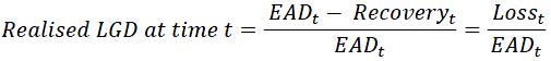
4.3.5
The recovery is derived from all cash inflows and expenses occurring at future times after the default event and discounted back to the default date. The recovery cash flows should not be higher than the amount of recoveries that can legally be obtained by the institution. The discount rates should reflect the time-value of money plus the uncertainty surrounding the cash flows. Additional considerations for restructured facilities are presented at the end of this section. If several facilities are secured by one or several collaterals, institutions should implement a clear collateral allocation mechanism from the obligor level to each facility. The computations of Recoveryt and Losst depend on the workout outcome. The estimation method should incorporate the following components.
Table 4: Recovery and costs per type of outcome
Outcome Components of recovery and costs (1) Cured & not restructured (a)
Indirect costs, as defined in the data collection section.
(2) Cured & restructured (a) Potential reduction in present value upon restructuring the facility. (b) Direct costs, as defined in the data collection section. (c)
Indirect costs, as defined in the data collection section.
(3) Not cured & secured (a) When applicable, present value of discounted collateral proceedings back to the default date (b) Direct costs, as defined in the data collection section. (c) Indirect costs, as defined in the data collection section. (d)
Cash flows received but not associated with collateral liquidation.
(4) Not cured & unsecured (a) Recovered cash flows. Effect of discounting these cash flows back to the default date, function of the time to recovery. (b)
Indirect costs, as defined in the data collection section.
(5) Unresolved These should be treated as per the following article. 4.3.6
The treatment of unresolved default cases (incomplete workouts) creates a material bias in the estimation of LGD. Consequently, institutions should establish a clear process for the treatment of these cases and understand their impact on the estimation of historical realised LGD.
(i)
Institutions should define criteria to decide on whether the recovery process of a default case should be considered closed. A degree of conservativeness should be included in this estimation to reflect the uncertainty of the recovery process. This means that if doubts persist regarding the possibility of future cash inflows, the recovery process should be considered closed. (ii)
Institutions should put in place clear criteria to include or exclude unresolved cases in their estimation samples. For that purpose, a maximum length of resolution period (from the date of default) should be established by obligor segment. The objective is to choose a duration that is sufficiently short to maximise the number of recovery cases flagged as ‘closed’ and sufficiently long to capture a fair recovery period. (iii)
It is recommended that open default cases with a recovery period longer than four (4) years should be included in the LGD estimation process, irrespective of whether they are considered closed. For the avoidance of doubt, all closed cases with a shorter recovery period should, of course, be included. Banks are free to use a shorter maximum duration. Longer maximum duration, however, should be avoided and can only be used upon robust evidence provided by the institution. (iv)
Default cases that are still unresolved within the maximum length of the recovery process (i.e. shorter than 4 years) should preferably be excluded for the purpose of estimating historical LGDs. Institutions have the option to consider adjustments by extrapolating the remaining completion of the workout process up to the maximum resolution period. Such extrapolation should be based on documented analysis of the recovery pattern by obligor segment and/or product type observed for closed cases. This extrapolation should be conservative and incorporate the possibility of lower recovered cash-flows.
Table 5: Treatment of unresolved default cases
Recovery status Shorter recovery than the maximum recovery period Longer recovery than the maximum recovery period Closed cases Included. All discounted cash-flows taken into account. Included. All discounted cash-flows taken into account. Open cases Excluded. Possible inclusion if cash-flows are extrapolated. Included. All discounted cash-flows taken into account. 4.3.7
Institutions should not assume that restructuring and rescheduling events necessarily lead to zero economic loss. For restructuring associated with material exposures, an estimation of their associated present value impact should be performed. If no PV impact is readily available, then the terms of the new and old facilities should be collected in order to estimate a PV impact, according to the methodology outlined in the dedicated section of the MMG. In particular, if the PV impact of the cash flow adjustment is compensated for by a capitalisation of interest, institutions should include an incremental credit spread in discounting to reflect the uncertainty arising from postponing principal repayments at future dates. Such credit spread should then lead to a negative PV impact.
4.3.8
For low default portfolios, institutions may not have enough data to estimate robust historical recovery patterns. In this case, institutions should be in a position to demonstrate that data collection efforts have taken place. They should also justify subsequent modelling choices based on alternative data sources and/or comparables. Furthermore, portfolios with high frequency of cure via restructuring should not be considered as portfolios with low default frequency. Restructured facilities could be recognised as defaults depending on circumstances and in compliance with the CBUAE Credit Risk Regulation.
4.4 Analysis of Realised LGD
4.4.1
Once institutions have estimated and categorised realised LGD, they should analyse and understand the drivers of realised LGD in order to inform modelling choices in the subsequent step.
4.4.2
At a minimum, institutions should analyse and understand the impact of the following drivers on LGD:
(i)
The time at which LGD was observed in the economic cycle. The profile of the recovery pattern and the effect of the economic cycle on this pattern. (ii)
The effect of collateral on the final LGD including the time to realise the collateral, the impact of the type of collateral, the difference between the last valuation and the liquidation value. (iii)
The link between LGD and the obligor’s credit worthiness at the time of default captured by its rating or its PD. (iv) The type of facility and its seniority ranking, where applicable. (v) The obligor segments expressed by size, industry, and/or geography. (vi)
Any change in the bankruptcy legal framework of the jurisdiction of exposure.
4.4.3
Institutions should identify the most appropriate segmentation of historical realised LGD, because this choice will subsequently inform model segmentation. Portfolio segmentation should be based upon the characteristics of the obligors, its facilities and its collateral types, if any.
4.4.4
Institutions should be cautious when using ‘Secured LGD’ and ‘Unsecured LGDs’ as portfolio segments. A secured LGD is a loss obtained from a facility secured by a collateral. It is based upon the estimation of a collateral coverage (defined as the ratio of the collateral value to the exposure). The loss resulting from such coverage can spread across a large range: from low values in the case of over-collateralization, up to high values in the case of small collateral amounts. An average (referred as Secured LGD) across such large range of values is likely to suffer from a lack of accuracy. Thus, it is preferable to employ collateral as a direct continuous driver of LGD, rather than use it to split a population of obligors.
4.4.5
Once segments have been identified, institutions should produce three types of LGD per segment to support the estimation of ECL as per accounting principles. These estimates should be used to calibrate the TTC LGD and PIT LGD models in subsequent modelling steps. The estimation of averages can be exposure-weighted or count-weighted. This choice depends on each portfolio and thus each institution.
(i)
The long run average by segment, through time across business cycles, estimated as the average of realised LGDs over the observation period. (ii) The LGD during economic downturns. (iii)
The LGD during periods of economic growth.
4.4.6
When analysing the effect of collateral on LGD outcomes, institutions should consider, at a minimum, the following collateral types. Note that personal guarantees should not be considered as eligible collateral for the purpose of modelling LGD. This list may evolve with the CBUAE regulation.
Table 6: Types of eligible collateral
Collateral types Cash (or cash equivalent) Federal Government (security or guarantee) Local Government (security or guarantee) Foreign sovereign government bonds rated BBB- or above UAE licensed Bank (security or guarantee) Foreign bank rated AA- or above (security or guarantee) Foreign bank rated BBB- but below AA- (security or guarantee) Listed Shares on a recognized stock exchange Bonds or guarantees from corporations rated above BBB- Residential Real Estate Commercial Real Estate All other banks bonds or guarantees Cars, Boats, Machinery and other movables All other corporate bonds or guarantees (not including cross or personal guarantees) 4.5 TTC LGD Modelling
4.5.1
The objective of TTC LGD models is to estimate LGD, independently of the macroeconomic circumstances at the time of default. Therefore, these models should not depend on macroeconomic variables. These models can take several forms depending on the data available and the type of portfolio. Institutions are free to choose the most suitable approach, provided that it meets the minimum expectations articulated in this section.
4.5.2
Defaulted vs. non-defaulted cases: LGD should be modelled and estimated separately between defaulted obligors (or facilities) and non-defaulted obligors. Whilst the methodology should be similar between these two cases, several differences exist:
(i)
Upon a default event, the estimation of recovery relies on assumptions and on a live process with regular information updates. Therefore, for defaulted obligors (or facilities), as the recovery process unfolds, institutions should collect additional information to estimate recovery rates with further accuracy and thus obtain more specific LGD estimation. (ii)
For defaulted obligors (or facilities), particular attention should be given to PV modelling as per the dedicated section of the MMG. Discount factors should reflect the circumstances of default and the uncertainty surrounding the recovery process. (iii)
One of the major differences between LGD from defaulted vs. non-default exposures is that the former is estimated only as of the date of default, while the latter is estimated at several point in time, depending on the needs of risk management and financial reporting.
4.5.3
Properties: At a minimum, LGD models should meet the following properties.
(i)
The modelled LGD should be based upon the historical realised LGD observations previously estimated. (ii)
The methodology should avoid excessive and unreasonable generalisations to compensate for a lack of data. (iii)
The model performance should be validated based on clear performance measurement criteria. For instance, model predictions should be compared against individual observations and also against segment average. (iv)
There should be enough evidence to demonstrate that in-sample fit and out-of-sample performance are reasonable. (v) The choice of parameters should be justified and documented. (vi)
The model inputs should be granular and specify enough to generate a LGD distribution that is a fair and accurate reflection of the observed LGDs.
4.5.4
Functional form: Institutions are free to use LGD models with any functional form provided that the model output is an accurate reflection of the observed LGD. Institutions should aim to build LGD models that incorporate the suitable drivers enabling the model to reflect the main possible outcomes of the workout process.
4.5.5
Parameters: Institutions should aim to incorporate the following drivers in their LGD models. This means that any model using less granular inputs should be considered as a first generation model that requires improvement as further data becomes available.
(i) The probability of cure without restructuring, (ii) The probability of cure through restructuring, (iii) The collateral coverage, (iv) Direct and indirect recovery costs, (v) Collateral liquidation values including haircuts, and (vi)
Recovered cash flows
The quantitative drivers above should be analysed (segmented) by qualitative drivers, including but not limited to:
(vii) Industry or obligor type, (viii) Facility type, and (ix)
Seniority ranking.
4.5.6
The parameters listed above should drive the estimation of LGD. The mathematical construction of the LGD model can take several forms, that institutions are free to choose. The form presented below serves as illustration. Institutions are not expected to use this expression literally; rather, they should ensure that their final LGD model respects the principles of this expression with a suitable estimation of each component. If institutions employ a different functional form, they are encouraged to use the following expression as a challenger model.

Table 7: Typical components of LGD models
Component Definition P1 Probability of cure without restructuring P2 Probability of cure through restructuring S Collateral coverage defined as 𝐶𝑜𝑙𝑙𝑎𝑡𝑒𝑟𝑎𝑙 𝑉𝑎𝑙𝑢𝑒 ⁄𝐸𝐴D L1 Loss (cost) from managing delinquent clients that were cured without restructuring L2 Loss from managing delinquent clients through restructuring or rescheduling, including direct and indirect costs plus NPV impacts. L3 Loss from the realisation of collateral including haircuts, direct and indirect costs plus NPV impact. Estimated across all collateral types. L4 Loss arising from the incomplete recovery of the portion of exposure not covered by collateral, also including indirect management costs and NPV impacts. (Referred to as unsecured LGD.)
The loss arising from the unsecured portion (L4) is often called "unsecured LGD". The final LGD after taking collateral into accounts is often referred to as the "secured LGD". Irrespective of the semantic employed, LGD models should reconcile conceptually against the expression above.
4.5.7
Granularity: Institutions should aim to develop TTC LGD models to estimate LGD at a low level of granularity. The following minimum expected practices apply:
(i)
Institutions should aim to model LGD at facility level, i.e. the LGD should incorporate facility characteristics. If this is not possible for practical reasons, LGD should be computed at obligor level. This means that LGD should be driven by parameters specific to each obligor and the associated collaterals if any. (ii)
If several facilities are secured by one or several collaterals, institutions should implement a clear collateral allocation mechanism from the obligor to each facility. (iii)
If institutions do not have the required data to build such granular models, they should put in place a formal project in order to collect the necessary data as a stepping stone towards accurate LGD modelling.
4.5.8
Segmentation: The portfolio segmentation employed to estimate LGDs should be justified and documented. In theory, LGD segments do not have to be identical to those employed for PD modelling. However, in practice, it is recommended to use similar portfolio segmentation across PD and LGD models, where possible, in order to ease the interpretation of LGD and subsequent usage in provision and capital estimation.
4.5.9
Collateral haircuts: The last valuation of an asset is unlikely to reflect the resale value of a repossessed asset. Consequently, institutions should estimate appropriate haircuts based on the assumption that they intend to sell the repossessed asset as soon as reasonably possible. Haircuts should be estimated based on historical data by type of collateral.
4.5.10
Bimodal distribution: Institutions should identify whether the distribution of observed LGD is bimodal, i.e. a distribution with two peaks of high frequency. In this case, specific modelling constraints apply. Institutions should be cautious when using an average value between these two peaks. Such average can be misleading and should not be employed to assign LGD at facility level since it does not correspond to an observable LGD at facility level.
4.5.11
Logical features: Following on from the conceptual framework presented above, some logical characteristics should be respected: (i) the final LGD should be equal or smaller than the unsecured LGD, (ii) the LGD should decrease with the presence of collateral, all other parameters being kept constant, and (iii) the longer the recovery period, the higher the recovery, the lower the LGD. The logical features should be tested as part of the model validation process.
4.6 PIT LGD Modelling
4.6.1
There is general evidence that LGD levels tend to be higher during economic downturns. This intuitive relationship is supported by numerous publications from academics and practitioners based on data from the US and European markets. In the UAE, whilst this relationship is more difficult to prove, there are objective reasons to believe it exists. In any case, this should be investigated as part of current accounting requirements. Consequently, institutions should implement a process to analyse the relationship between LGD and macro factors. This should be done at a relevant level of granularity.
4.6.2
This analysis should drive the modelling strategy of PIT LGD. Several modelling options can be envisaged and institutions should articulate explicitly their approach based on their preliminary analysis. While making a strategic decision, institutions should remain conservative. A portfolio may not be large enough to capture this relationship despite the existence of such relationship at larger scale. In doubt, it is preferable to include some degree of correlation between LGD and macro factors for the estimation of ECL. Once a mechanism is in place, the strength of the relationship can be adjusted in calibration exercises, upon further evidence proving or refuting it.
4.6.3
The objective of PIT LGD models is to estimate LGD as a function of the economic circumstances at the time of default and during the recovery process. Therefore, these models should depend on macroeconomic variables. Institutions are free to choose the most suitable methodology, provided that it meets the minimum expected practices articulated in this section.
4.6.4
PIT LGD models can be constructed by (i) adjusting TTC LGD or (ii) developing models independently from TTC LGD. For consistency purpose, the former is recommended over the latter. If institutions chose the second approach, they should ensure that both PIT LGD output and TTC LGD outputs are coherent.
4.6.5
The properties of the PIT LGD models should be similar to that of TTC LGD models. At a minimum, these models should meet the following:.
(i)
The modelled LGD should be based upon the historical realised LGD observations previously estimated. (ii)
The methodology should avoid excessive and unreasonable generalisations to compensate for a lack of data. (iii)
The model performance should be validated based on clear performance measurement criteria. For instance, model predictions should be compared against individual observations (or relevant groups) and also against segment average. (iv) The choice of parameters should be justified and documented. (v)
There should be enough evidence to demonstrate that in-sample fit and out-of-sample performance are reasonable. (vi)
The model inputs should be granular and specify enough to generate a PIT LGD distribution that is a fair and accurate reflection of the observed LGDs.
4.6.6
PIT LGD models can take several forms depending on the data available and the type of portfolio. Several broad categories of models can be defined as follows, ranked by increasing granularity and accuracy:
(i)
Option 1: Most granular approach. The LGD parameters are directly linked to the macro forecasts and used as inputs to compute the losses (L1,L2,L3,L4). The final LGD is subsequently computed based on these losses, as defined in the TTC LGD section. For instance, collateral values at facility level can be directly linked to the macro forecasts, then secured LGDs are derived. (ii)
Option 2: Intermediate granular approach. The losses (L1,L2,L3,L4) are linked to the macro forecasts and used as input to estimate the final LGD, as defined in the TTC LGD section. For instance, the segment level secured and unsecured LGDs can be linked to the macro forecasts. (iii)
Option 3: Non-granular approach. The final LGD is directly linked to the macro forecasts. In this case the PIT LGD models does not use the LGD parameters. (iv)
Option 4: Alternative approach. The final LGD is linked to the obligor's PD, itself linked to macro forecasts. In this case, the LGD response to macroeconomic shocks is constructed as a second order effect through correlation rather than structural causation.
4.6.7
Institutions should articulate and document explicitly their preferred modelling option. All these options are acceptable; however institutions should be aware of their theoretical and practical limitations, in particular the potential accuracy issues arising from options 3 and 4. Institutions should aim to model PIT LGD via option 1. Consequently, institutions should understand and assess the financial implications of their modelling choice. This choice should be approved by the Model Oversight Committee.
4.6.8
If the PIT LGD model uses PIT PD as a sole driver of macro adjustment, then the model segmentation should be identical between PIT LGD and PIT PD. If institutions decide to develop dedicated PIT LGD-macro models, those should follow the minimum expectations articulated in the section of the MMG dedicated to macro models.
4.7 Validation of LGD Models
4.7.1
Institutions should validate all LGD models according to the validation principles articulated in the MMS. Both qualitative and quantitative assessments should be conducted for an appropriate validation.
4.7.2
Institutions should ensure that segment-level LGD values represent the risk profile of their books. Statistical tests alone are not sufficient to conduct appropriate validation of LGD at segment level. Consequently, institutions should combine statistical tests, judgement and checks across comparable metrics to ensure that the calibration of these metrics are meaningful and accurate.
4.7.3
The scope of the validation should be comprehensive. If the validation is performed by a third party consultant, institutions should ensure that the validation effort is comprehensive in scope and substance.
4.7.4
The validation scope should include, at a minimum, the following components:
(i)
The data quality, comprehensiveness and collection process. This should cover the analysis of unusual features observed in historical data and their subsequent treatment for modelling. (ii)
The definition of default. This should cover the treatment of technical defaults and restructured accounts. (iii)
The methodology employed to compute historical LGD. This should cover in particular the possible outcomes as described earlier in this section. Partial replication of the historical LGD for a sample of facilities should be performed. (iv)
The methodology employed to estimate TTC LGD and subsequent PIT adjustments. This should cover the model fit, functional form, robustness, properties and sensitivities. (v)
The treatment of collateral. The treatment of LGD segmentation granularity. The quality of the model output in terms of economic and business meaning. This can rely on comparables based on data available outside of the institution. (vi)
The existence of spurious accuracy and excessive generalisation. In particular, the validation process should report the excessive usage of average LGD employed across a large population of heterogeneous obligors. (vii)
Back-testing of modelled LGD, estimated separately for defaulted and non-defaulted obligors.
5 Macroeconomic Models
5.1 Scope
5.1.1
Macroeconomic models (“macro models”) are primarily employed by UAE institutions for the estimation of Expected Credit Loss (“ECL”) and for internal and regulatory stress testing purpose. The objective of this section is to provide guidance and set the Central Bank’s expectation applicable to all macroeconomic models used by institutions. The practices described in this section are in compliance with current accounting principles.
5.1.2
In this context, macro models are defined as statistical constructions linking macro variables (“independent variables”) to an observed risk or business metrics, typically PD, Credit Index, LGD, cost of funds, or revenues (“dependent variables”). Several types of macro models exist. A common approach relies on time series regression techniques, which is the main focus of this section on macro models. Other approaches include (i) for retail clients, vintage-level logistic regression models using directly macroeconomic drivers as inputs and (ii) for corporate clients, structural models using macro variables as inputs.
5.1.3
Irrespective of the methodology employed, institutions should use judgement and critical thinking, where statistical techniques are coupled with causality analysis. Institutions should justify and balance (i) statistical performance, (ii) business intuition, (iii) economic meaning, and (iv) implementation constraints. Statistical methods and procedures will only provide part of the solution. Therefore, rigorous modelling techniques should be coupled with sound economic and business judgement in order to build and choose the most appropriate models. The key modelling choices and the thought process for model selection should be rigorously documented and presented to the Model Oversight Committee.
5.1.4
The modelling decision process should be driven by explorations, investigations, and comparisons between several possible methods. Note that time series regression models have been proven to yield the most intuitive results over other techniques.
5.1.5
When developing macro models, institutions should follow a clear sequential approach with a waterfall of steps. Depending on the outcome, some steps may need to be repeated. Each step should be documented and subsequently independently validated. In particular, for time series regression models, the process should include, at a minimum, the steps presented in the table below.
Table 8: Sequential steps for the development of macro models
# Step 1 Data collection 2 Analysis of the dependent variables 3 Analysis of the macro variables 4 Variable transformations 5 Correlation analysis 6 Model construction 7 Statistical tests 8 Model selection 9 Monitoring and validation 10 Scenario forecasting 5.2 Data Collection
5.2.1
In order to proceed with macroeconomic modelling, institutions should collect several types of time series. This data collection process should follow the requirements articulated in the MMS.
5.2.2
At a minimum, these time series should be built with monthly or quarterly time steps over an overall period of five (5) years covering, at least, one economic cycle. Institutions should aim to build longer data series. The following data should be collected.
5.2.3
Macro variables: Institutions should obtain macro variables from one or several external reliable sources.
(i)
The scope of variables should be broad and capture appropriately the evolution of the economic environment. They will typically include national accounts (overall and non-oil, nominal and real), oil production, real estate sector variables, CPI, crude oil price and stock price indexes. (ii)
Institutions should collect macro data pertaining to all jurisdictions where they have material exposures (at least greater than ten percent (10%) of the total lending book, excluding governments and financial institutions). (iii)
Institutions should document the nature of the collected variables, covering at a minimum, for each variable, a clear definition, its unit, currency, source, frequency, and extraction date. (iv)
Institutions should ensure that all variables employed for modelling will also be available for forecasting.
5.2.4
Historical default rates: Macro-PD models (or macro-to-credit index models) stand at the end of a chain of models. They are employed to make adjustments to the output of TTC PD models, themselves linked to rating models. Therefore the default data used for macro-PD modelling should reflect the institution’s own experience. If external default data points are used, justification should be provided. Finally, institutions are encouraged to also include restructuring and/or rescheduling events in their data to better capture the relationship between obligor creditworthiness and the economic environment.
5.2.5
Historical recovery rates: Macro-LGD models are designed to adjust the output of TTC LGD models. Consequently, the recovery data employed for macro-LGD modelling should reflect the institution’s own experience. If external recovery data points are used, justification should be provided.
5.2.6
Macro data series are mostly available with quarterly or even annual data points and rarely with monthly time intervals. Consequently, interpolation techniques may need to be developed. Institution should include interpolation methodology as part of the data transformation step. Such interpolation should be documented and included in the validation process.
5.3 Analysis of the Dependent Variables
5.3.1
Institutions should demonstrate that default series are suitable for modelling and are representative of their current portfolio. For that purpose, they should employ judgement and critical thinking when analysing the data. At a minimum, they should perform an analysis of the dependent variables through descriptive statistics, covering the distribution followed by each dependent variable and the identification of outliers, if any. Upon this analysis, a clear statement should be made regarding the suitability of the data for macro modelling. Consideration should be given to (i) the data quality, (ii) length, and (iii) representativeness. This analysis should be fully described in the model development documentation.
Business consistency: Institutions should pay attention to the business significance of the historical data related to the dependent variable. One possible conclusion is that historical data of a given variable is no longer an appropriate representation of the current institution’s portfolio because the segment business strategy has changed materially. In the case of default and recovery rates, conservatism prevails.
(i)
The institution may believe that its current portfolio is less risky than its historical portfolio and that it expects to experience lower default rates and/or losses in the future. In that case, the existing historical default series should be used for a reasonable period until there is enough evidence supporting the new risk profile. Subsequently, adjustments are permitted on the forecasted values, for instance in the form of scalers. (ii)
The institutions may believe that its current portfolio is more risky than its historical portfolios and that it will consequently experience higher default rates in the future. In that case, forecasts should be immediately adjusted, i.e. forecasted PDs and LGDs should be shifted upward.
5.3.2
Regime shifts: Institutions should identify the presence of regime shifts in all times series. These can be clearly identified by the presence of sudden permanent jumps in the data. Regime shifts tend to occur in default and recovery series due to changes in the data collection process, definition of default, recovery process or business strategies. For modelling, it is strongly recommended to avoid using time series with regime shifts as direct model inputs. Instead, adjustments should be implemented such as a truncation of the series or the use of specific econometrics techniques (the introduction of a dummy variable in the model).
5.3.3
Segmentation consistency: Segmentation means splitting a statistical sample into several groups in order to improve the accuracy of modelling. This concept applies to any population of products or customers. In particular, for the construction of PD and LGD macro models, the choice of portfolio, customer and/or product segmentation has a material impact of the quality of macro models. The economic behaviours of obligors and/or products should be homogeneous within each segment in order to build appropriate models. As mentioned in the data collection section, a degree of consistency is required between macro models and other models. For macro-PD models in particular, such consistency should be analysed and documented as follows:
(i)
The granularity of segments for macro modelling should be equal or greater than the granularity of segments employed for (i) rating models, and (ii) PD term structures models. If this alignment is not possible, institutions should provide robust justifications and document them accordingly. (ii)
Institutions may decide to increase the segmentation granularity of macro models. An increase in the number of segments will lead to a reduction in segment size and in the number of observed defaults, could, in turn, reduce the statistical significance of the default rate. Therefore, increasing the segmentation granularity is permitted, provided that there is no material loss in the representativeness of the default rates.
5.3.4
Institutions should analyse and assess the impact of segmentation choices as part of the development of macro models. Several segmentation options should be considered and subject to the entire model development process described hereby. Institutions should then choose the best segmentation by assessing the quality and robustness of the macro models across several segmentation options.
5.4 Analysis of the Macro Variables
5.4.1
Institutions should perform a robust analysis of the macro variables through descriptive statistics. At minimum, this analysis should examine, amongst others, the shape of distribution to identify outliers, shape of tails, multimodality. Upon this analysis, a clear statement should be made regarding the suitability of the data for macro modelling. In particular, the analysis should consider the data quality, length and representativeness. This analysis should be fully described in the model development documentation.
5.4.2
Regime shift: Institutions should identify the presence of regime shifts in all macro time series. Regime shifts can occur in macro time series due to economic decisions such as the introduction of VAT or a large shift in interest rates. Similarly to the dependent variables, macro time series with regime shifts should be avoided or adjusted accordingly.
5.4.3
Economic consistency: Institutions should pay attention to the economic significance of the macro variables. Some macro variables provide consistently better explanatory power of risk metrics in the banking book. Conversely some variables are more challenging to interpret, consequently institutions should be cautious when using those variables for PD and LGD macro models. Particular attention is needed for the following:
(i)
Employment rate: A large proportion of employees leave the UAE upon losing their employment. Consequently, the UAE employment rate incorporates a material bias, hence it is preferable to avoid this variable to model business or risk metrics. (ii)
Interest rates: The relationship between interest rates and default rates is ambiguous. Institutions should ensure that an appropriate interpretation of the estimates is provided upon modelling PDs and LGDs. (iii)
Abu Dhabi and Dubai stock indices: These indices can suffer from a lack of liquidity therefore institutions should ensure that an appropriate interpretation of the estimates is provided upon modelling PDs and LGDs. (iv)
UAE account balances (e.g. fiscal balance, current account): By construction these variables can oscillate between positive and negative values. Consequently, a relative time differencing can lead to very high returns and uncontrollable spikes. Instead, it is recommended to normalise these variables by nominal GDP prior to using them for modelling.
5.5 Variable Transformations
5.5.1
The principles of variable transformation articulated in the MMS also apply to macro models. Variable transformations have a material impact on macro models and on ECL. Therefore, institutions should test, choose and document the most appropriate transformations applied to both the macro variables and to the dependent variable.
5.5.2
Stationarity: Modelled economic relationship should be stable over time. In the context of time series regression model, variables should be stationary in order to construct robust and meaningful econometric models. Stochastic trends, seasonality and structural breaks are most common sources of non-stationarity. This property should be tested for both the dependent and independent variables, according to the following principles:
(i)
Macroeconomic variables should meet stationarity criteria prior to be used for modelling. The absence of stationarity has adverse material consequences on macro models because it often leads to spurious correlations. Macro variables that are not stationary should either be transformed to obtain stationary series or should be excluded from the modelling process. (ii)
Even after transformations, in some circumstances full stationarity is challenging to obtain if series are short and data is scarce. In this case, institutions should use judgement and critical thinking to balance economic significance and stationarity requirement in order to assess if modelling can proceed. In this assessment, institutions should pay particular attention to the presence of trends, that often leads to spurious correlations. (iii)
To test for stationarity, standard unit root test may be used, including the Augmented Dickey-Fuller test, the Phillips-Perron test, the Kwiatkowski-Phillips-Schmidt-Shin (KPSS test). In case there is evidence of the presence of stochastic trend, standard transformations can be applied such as quarter-on-quarter or year-on-year log differencing. (iv)
Seasonality may be checked using X12 or X13 seasonal adjustment algorithms. Year-on-year differencing could also be used to remove stable seasonal patterns. Formal structural breaks tests (e.g. Chow test) may be employed if there is visual evidence of break in the series. (v)
Common stochastic trends between two variables may be explicitly modelled using the rigorous application of standard co-integration models (e.g. Engle-Granger two step method or Johansen approach). (vi)
The absence of stationarity of the dependent variable can also be addressed by a first order time differencing or by autoregressive models. However, this can potentially lead to further complexity in implementation. Institutions should use judgement in this choice provided that it is justified and clearly documented.
5.5.3
Differencing: Time differencing should be based upon the following principle. Let Xt be a time series of the macroeconomic variable X at regular time steps t. Formally we can define two types of changes: (i) backward looking returns that estimate the change of the variable over a previous horizon h and (ii) forward looking returns that estimate the change of the variable over a coming horizon h. Formally:
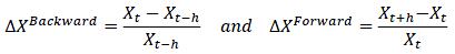
It is recommended to build macro models based on backward looking returns as these are more intuitive to interpret and easier to implement. It is also recommended to compute backward looking default rates in order to ensure that both the dependent and independent variables are homogeneous.
5.5.4
Horizon of differencing: Institutions should choose carefully the horizon of return applied to macro variables, i.e. the period used to compute the change of a variable through time. Institutions should take notes of the following principles:
(i)
For macroeconomic models, common return horizons include quarterly, half-yearly and yearly. The most appropriate return horizon should be chosen to maximize the explanatory power of the macro variables. (ii)
Note that the return horizon is not necessarily equal to the granularity of the time series. For instance, rolling yearly returns can be computed on quarterly time steps. (iii)
Institutions should be aware of the degree of noise in high frequency data. Consequently judgement should be used when using high frequency returns.
5.5.5
Lags: Variable lags should be considered in the modelling process to capture delayed effects of macro drivers. The use of large lags (more than 6 quarters) should be justified since long lags delay the impact of macro shocks on the dependent variable. For each macro variable, the choice of the most appropriate lag should be based on its statistical performance and economic meaning.
5.5.6
Smoothing: This means reducing the presence of spikes and outliers in times series. This is commonly addressed by the usage of moving average. Such practice is permitted but should be employed with caution and documented. The right balance of smoothing needs to be found. No smoothing (too much noise) in time series can lead to weak models. Alternatively, too much smoothing can dilute the strength of correlations. Smoothing techniques should be documented when applied.
5.5.7
Standard and intuitive transformations should be used. For example, the growth rate of a variable that can be zero or negative is not a meaningful measure.
5.6 Correlation Analysis
5.6.1
The objective of the correlation analysis is to assess the strength of the relationship between (i) each of the transformed dependent variable (e.g. PD) and (ii) each of the transformed macro variables, on a bilateral basis. Consequently such univariate analysis should be performed for each obligor segment. This analysis should include both statistical and causality perspectives. Relationships should make economic sense and meet business intuitions.
5.6.2
Institutions should pay attention to the strength and sign of correlations (positive vs. negative relationships) and assess whether they meet business intuitions. At a minimum, the following components should be documented: (i) the top macro variables ranked by correlation strength and (ii) comments and analysis on the observed statistical relationships vs. expected business intuitions.
5.6.3
A cut-off should be establish to eliminate the transformed macro variables that display weak and/or incoherent correlations with the independent variables. This reduced population of transformed macro variables should be used to perform multivariate analysis.
5.7 Model Construction
5.7.1
The objective of this step is to construct relevant and robust relationships between a single transformed dependent variable (e.g. PD) and several macro variables. The choice of the macro variables entering each model should be based upon the results of the correlation analysis. This process results in the construction of a range of multifactor models for each dependent variable.
5.7.2
In the context of time series regressions, institutions should choose the most appropriate methodology to perform multifactor regressions. Amongst others, it is recommended to perform multifactor regressions with or without autoregressive terms. It is recommended that institutions include several modelling forms as part the pool of possible model candidates.
5.7.3
The estimation of model coefficients should be performed with recognised professional statistical software and packages. The entire process should be fully documented and replicable by an independent party.
5.7.4
Several performance metrics should be used to rank and choose models. As these metrics depend on the type of models, institutions should use judgements to employ the most appropriate performance metrics per model type. At a minimum, the adjusted R-square should be used for multifactor regression models. For models based on the ARIMA form, a pseudo R-square should be employed as the square of the correlation between the fitted variable and the original dependent variable.
5.8 Statistical Tests
5.8.1
Standard post-estimation tests should be used to check that the underlying assumptions are appropriate for all types of macro models. The set of appropriate tests should be based on best practices in the relevant field / literature. The model development documentation should clearly indicate (i) the chosen test for each property, (ii) the nature of the H0 hypothesis, (iii) the cut-off values chosen upfront to determine the rejection or non-rejection.
5.8.2
In the context of time series regression, regression coefficients should be significant and residuals should be tested for autocorrelation and normality. The table below indicates properties that should be tested, at a minimum. Other tests may be considered, if necessary.
Table 9: Typical statistical tests for models based on time series regression
Property to be tested Description of the property to be rejected Suggested test (others may exist) Stationarity Absence of stationarity in each time series Augmented Dickey-Fuller (ADF) Co-integration Absence of stationarity in a linear combination of the dependent variable and each independent variable Engle-granger two-step method Multicolinearity High correlation between the independent variables Variance Inflation Factor Coefficient significance The coefficients are not statistically significantly different from zero Coefficient p-value on a t-distribution Autocorrelation High correlation between the error terms of the model Ljung-Box test Heteroscedasticity Absence of relationship between independent variables and residuals Breusch-Pagan or White test Normality Normal distribution of the residuals Shapiro Wilk 5.9 Model Selection
5.9.1
The model and macroeconomic variable selection should be based on clearly defined performance criteria using a transparent selection algorithm. The final model should be able to (i) generate values that fit the historical values of the dependent variable and (ii) generate accurate predictions.
5.9.2
For each segment, institutions should choose a final model from the list of candidate models generated from the model construction step. Statistical performance should not be the only decisive factor to choose a model. Instead, the choice of the final model should be based upon the combination of various factors. At a minimum, institutions should use the criteria outlined below. It is essential that institutions include all these criteria in the selection process. The absence of one criteria could be materially detrimental to the choice of the most relevant model.
(i)
Statistical performance:
a.
The chosen model should meet minimum requirements of performance, statistical stability and robustness as shown by the statistical indicators and their associated thresholds. Model parameters and forecasts should remain stable over time. b.
In addition, at the model development stage, it is important to examine the stability of models: out-of-sample performance and in-sample fit should be tested and compared across candidate models. A common metric employed to express model performance is the root mean square error, for which limits should be established.
(ii)
Model sensitivity: Quantitative response of the dependent variable to independent variables should be meaningful and statistically significant - both quantitatively and qualitatively. This can be examined through simulating one standard deviation change in individual dependent variables or by considering the forecast differences across alternative scenarios. (iii)
Business intuition: The chosen model should be constructed with variables and relationships that meet logical business and economic intuitions. This means that the model should be explained by causal relationships. (iv)
Realistic outcomes: Projected values should be consistent with historical observations and meet economic intuition. Any material jump and/or disconnect between historical values and forecasted should be explained. (v)
Implementation: When choosing a model, institutions should be mindful of the implementation and maintenance constraints, which should form part of the choice of the most appropriate models. For instance, some variables may not be available as frequently as expected for forecasting. Also, some model formulations may require autoregressive terms that need specific treatment during implementation.
5.9.3
In order to test the business intuition, for each candidate model, institutions should forecast the dependent variables (e.g. PD, Credit Index) under a severe downside scenario. The outcome will therefore be a range of projected dependent variables (one for each model) under the same scenario. It may become apparent that some candidate models should be excluded as they generate outputs that deviate too much from economic and business expectations.
5.9.4
Forecast Uncertainty: Projected forecast are based on mean or median values, around which uncertainty (i.e. confidence interval) inherently exists. Institutions should ensure that the model forecast uncertainty are clearly estimated, documented and reported to the Model Oversight Committee. In the context of time series regression, the confidence interval around the mean can be estimated empirically or based on the standard deviation of the residuals under the assumption of normally distributed residuals.
5.10 Validation of Macro Models
5.10.1
The validation of macro models should be performed by a different and independent party from the development team, according to the validation principles articulated in the MMS. If macro models are developed by a third party consultant, then a team within the institution or another consultant should therefore perform these independent validations.
5.10.2
Monitoring macro models may be challenging due to the low frequency of macroeconomic data. Institutions are expected to monitor the performance of macro models once a year. However, exceptional monitoring is required in the case of exceptional macroeconomic events.
5.10.3
Pre-implementation validation: This step involves the validation of the chosen macro models immediately after their development, prior to using them in production. The objective is to ensure that macro models meet a minimum level of quality and that they are fit for purpose. At a minimum, the following validation steps should be performed.
(i)
Development process: The validator should review the development process as per the principles articulated in the MMS. (ii)
Replication: The validator should replicate the final chosen model per segment and ensure that the coefficients are correctly estimated. (iii)
Statistical tests: The validator should ensure that statistical tests are correct, that cut-offs are reasonable and that statistical assumptions are correctly interpreted. This may necessitate partial replication. Additional statistical tests may be needed. (iv)
Model sensitivity: The validator should measure the elasticity of the model output to changes in each input variable. The model user and validator should be aware of the presence of independent variables that dominates other variables in a given model. (v)
Model stability: The validator should test the model stability, for instance by removing data points from the original time series (at the start or the end), re-run the regressions and re-project the dependent variable. The validator should also examine the stability of the model coefficients. (vi)
Conclusion: When deemed appropriate, the validator can make suggestions for defect remediation to be considered by the development team.
5.10.4
Post-usage validation: This is otherwise referred to as back-testing, whereby the validator should compare the realized values of the dependent variable (e.g. PD, LGD, Credit Index) against the forecasted values based on the macroeconomic scenarios employed at the time of the forecast. A conclusion should be made based pre-defined confidence intervals.
5.10.5
Upon the post-usage validation, the validator should make a clear statement regarding the suitability of the model to be used for another cycle. When deemed appropriate, the validator can make suggestions for defect remediation to be considered by the development team.
5.11 Scenario Forecasting
5.11.1
The expected practices articulated in this section relate to the regular estimation of ECL. As per current accounting requirements, institutions should estimate an unbiased and probability weighted ECL by evaluating a range of possible outcomes. Consequently, institutions should forecast economic conditions over the lifetime of their portfolio. All the macroeconomic variables employed as input in macro models should be forecasted until the longest maturity date of the institutions’ portfolio.
5.11.2
Institutions are encouraged to disclose macroeconomic scenarios in their annual reports. For this information to be meaningful, institutions should provide the values of the main economic drivers over the next three (3) years with the weight of each scenario.
5.11.3
Institutions should use the most recent set of models to forecast PD and LGD. If the most recent models are not used in the computation of ECL, this should be mentioned in monitoring and validation reports and reported to internal and external auditors because it has direct impacts on financial reporting.
5.11.4
Governance: Institutions can either develop macroeconomic forecasts internally or rely on third party providers. In both cases, a governance process should be put in place to guarantee the quality of forecasts.
(i)
If scenarios are developed internally, they should be constructed by subject matter experts with robust economic knowledge, within the institution. The scenarios should be reviewed by the Model Oversight Committee and the committee in charge of ECL oversight. (ii)
If scenarios are developed externally, institutions should put in place an internal validation process, by which the forecasts are checked, errors are adjusted and economic consistency is ensured. Even if scenarios are provided by an external party, each institution remains the owner of the economic forecasts and therefore remains accountable for inconsistencies present in those scenarios. (iii)
To support the adequate estimation of ECL, institutions should produce regular reports to present the aspects of macro scenario calibration discussed in this section. The report should address the source of scenarios, their economic consistency, their severity, weights and potential adjustments.
5.11.5
Weights and severity: As per current accounting requirements, institutions should use several weighed scenarios. At a minimum, institutions should employ one base, one upside and one downside scenario for each macro variable. In order to obtain an unbiased estimation of ECL, both the scenario weights and their associated severity should be jointly calibrated. For each variable, institutions should pay attention to the relative weight and severity of the downside scenario vs. the weight and severity of the upside scenario. Finally, it is recommended to estimate the ECL under each scenario in order to convey possible ECL volatility and support appropriate risk management.
5.11.6
Forward looking information: As per current accounting requirements, ECL should be based on forward looking information that is relevant reasonable and supportable. This should be understood as follows:
(i)
The economic information should be based on consensus, when possible, rather than a single source. (ii)
The economic forecasts should be realistic in terms of trend, level and volatility. For instance, economic forecasts assuming a constant positive inflation should not push asset prices to excessive and unrealistic levels in the long term. This feature is particularly relevant for real estate collaterals. (iii)
The divergence between the scenarios (base, upside, downside) should meet economic intuition and business sense. Such divergence should follow a logical economic narrative.
5.11.7
Benchmarks: Aside from ECL measurement, institutions employ existing scenarios for planning purposes, with varying severity and probability of occurrence. Amongst others, dedicated scenarios are used for the ICAAP, the recovery and resolution plan, and for stress testing purpose. These scenarios should not be employed as input for ECL computation because they do not represent an unbiased probability-weighted set of scenarios. Similarly, the macroeconomic scenarios provided by the CBUAE as part of regulatory enterprise-wide stress testing exercises should not be used as input for ECL computation. All these alternative scenarios can only be used as distant comparables for the ECL scenarios. However, this comparison should be made with caution because the calibration (severity, likelihood) of the ECL scenarios is likely to be different.
5.11.8
The construction of the scenarios should be economically coherent and therefore should follow a set of rules to be consistent. Let Xt be a time series of the macroeconomic variable X at regular time steps t. For the purpose of articulating this point, we will use three scenarios. The time series of X corresponding to each scenario are noted Xtbase, XtUp and XtDown .
(i)
Scenarios should be constructed in such way that their values diverge after a given date, called the forecasting date, noted T. The time series for the three scenarios should be identical prior to the date of forecast and diverge after the date of forecast. Formally:
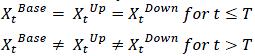
(ii)
The portfolio date noted K employed in loss computation should be close to the forecasting date. Therefore, institutions should keep updating the macroeconomic forecasts along with the portfolio date, in order to minimize the time difference between T and K. It may happen that ECL reporting is done at a higher frequency than the update of macroeconomic forecasts. In this case, the time step at which scenarios start diverging occurs before the portfolio date K. Formally, for T<K:

This misalignment is likely to create unwarranted effects in particular if scalers are used in PD modelling. Therefore, the maximum delay between the two dates should be no more than three months: K - T ≤ 3 months. If this difference is greater than three (3) months, the impact on the forecasted PD and LGD should be analysed and documented by the independent model validation team. (iii)
Beyond the forecasting start date, the upside and downside scenarios should not be constructed by a constant parallel shift (or scaling) of the base scenarios. Rather, the upside and downside scenarios should be constructed such that they display a gradual divergence from the base scenario through time (in growth rate terms if growth rates are applied). This property should apply to the stationary transformed macroeconomic variable. Consequently, the forecasted PD and LGD should follow the same pattern. Formally:
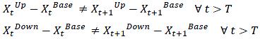
(iv)
Any scaler subsequently constructed based on these scenarios should follow the same pattern: a gradual divergence from the base scenario.
5.11.9
The principles articulated in this section about scenario forecast should also be included in the scope of review of the validation process. The validation process should test, assess and document practices for scenarios forecasts, including the governance, scenario construction and calibration.
6 Interest Rate Risk in the Banking Book
6.1 Scope
6.1.1
For the purpose of this section, and in order to simplify technical considerations, both interest rate risk (for conventional products) and profit rate risk (for Islamic products) will be referred to as Interest Rate Risk in the Banking Book (“IRRBB”). Both lead to a similar structural risk on institutions’ balance sheet.
6.1.2
Institutions should implement models to address the requirements articulated in “Interest rate and rate of return risk in the banking book Standards” issued by the CBUAE in 2018 (notice 165/2018), hereby referred to as the “CBUAE Standards on IRRBB”. In addition to the CBUAE Standards, institutions should refer to the Standards articulated by the Basel Committee on Banking Supervision in April 2016: “Interest rate risk in the banking book”, hereby referred as the “Basel Standards on IRRBB”.
6.1.3
According to the CBUAE Standards on IRRBB, interest rate risk should be captured through changes in both (i) expected earnings and (ii) the economic value of the balance sheet. In order to ensure more homogeneity in the methodology employed by institutions across the UAE, the MMG hereby presents some guidance on IRRBB modelling. The IRRBB requirements related to governance, management, hedging and reporting are covered in a separate CBUAE Standards on IRRBB.
6.2 Metrics
6.2.1
Institutions should identify all positions in interest sensitive instruments including:
(i)
All assets, which are not deducted from Common Equity Tier 1 (“CET1”) capital, and which exclude (a) fixed assets such as real estate or intangible assets and (b) equity exposures in the banking book. (ii) All liabilities, including all non-remunerated deposits, other than CE1 capital ; and (iii)
Off-balance sheet items.
6.2.2
Institutions should reconcile their exposures against their general ledger and their published financials. Differences may arise for valid reasons, which should be documented. This reconciliation process should be included in the model documentation and should be verified by the finance team on a yearly basis.
6.2.3
Changes in expected earnings and economic value can be captured through several possible metrics. At a minimum, the following metrics should be computed. These are referred as “IRRBB metrics”:
(i)
Gap risk: It is defined as the difference between future cash in-flows and cash-outflows generated by both assets and liabilities. The cash in-flows and out-flows are derived from the allocation of all relevant interest rate sensitive instruments into predefined time buckets according to their repricing or their maturity dates. These dates are either contractually fixed or based upon behavioural assumptions. The resulting metrics is the net position (gap) of the bank per future time bucket. (ii)
Gap risk duration: Also referred to as partial duration or partial “PV01”. It is defined as the modified duration of the gap per maturity bucket. The modified duration is the relative change in the present value of the position caused by a 1 basis point change in the discount factor in a specific maturity bucket. The resulting metrics is a term structure of PV01 per maturity bucket. (iii)
Economic value of equity: Also referred to as “EVE”. It is defined as the difference between the present value of the institution’s assets minus the present value of liabilities. The change in EVE (“∆EVE”) is defined as the difference between the EVE estimated with stressed discount factors under various scenarios, minus the EVE estimated with the discount factors as of the portfolio reporting date. (iv)
Net interest income: For the purpose of the MMG, and in order to simplify notations, both Net Interest Income (for conventional products) and/or Net Profit Income (for Islamic Products) are referred to as “NII”, defined as the difference between total interest (profit) income and total interest (profit) expense, over a specific time horizon and taking into account hedging. The change in NII (“∆NII”) is defined as the difference between the NII estimated with stressed interest rates under various scenarios, minus the NII estimated with the interest rates as of the portfolio reporting date. ∆NII is also referred to as earning at risk (“EAR”).
6.3 Modelling Requirements
6.3.1
The models employed to compute the metrics above should follow the principles articulated in the MMS. In particular all IRRBB models should follow the steps in the model life-cycle. The assumptions and modelling choices surrounding IRRBB models should not be the sole responsibility of the ALM function nor the market risk function. Rather, these assumptions should be presented to and discussed at the appropriate governance forum reporting to the Model Oversight Committee.
6.3.2
The modelling sophistication of the EVE should depend upon the size and complexity of institutions. For that purpose, different requirements are defined in function of their systemically important nature. The modelling requirements presented hereby should be regarded as minimum standards. To remain coherent with Basel principles, higher standards apply to large and/or sophisticated institutions (“LSI”). However, the other institutions may choose to implement models with higher standards than the one prescribed for them. This proportionality is an exception to the MMG due to the prescriptive nature of the Basel methodology surrounding IRRBB.
6.3.3
The requirements below refer to the methodology articulated in section IV (“The standardised framework”) of the Basel Standards on IRRBB. All institutions are requirements to fully understand this framework.
Table 10: Components of IRRBB models
Component LSIs Other institutions Computation
granularityFacility level or facility type if groups of facilities are homogeneous Summation of facilities within buckets, according to the Basel Standards Time buckets Granular bucketing depending on the composition of the books Standardised bucketing according to the Basel Standards on IRRBB Option risk Included in both EVE and NII Included in EVE
Optional from NIICommercial margins Optional from EVE
Included in NIIOptional from EVE
Included in NIIBasis risk Included Optional Currency Estimation for each material currency Estimation for each material currency Scenarios Standard plus other scenarios defined by institutions Standard six scenarios IT-system Dedicated system Spreadsheets can be used if the model and its implementation are independently validated 6.3.4
The estimation of EVE should be based upon the following principles: (a) it includes all banking book assets, liabilities and off-balance sheet exposures that are sensitive to interest rate movements, (b) it is based on the assumption that positions roll off, and (c) it excludes the institution’s own equity. The approach subsequently depends on the type of institutions.
(i)
LSIs should compute EVE as the difference between discounted assets and liabilities at a granular level. Institutions should aim to perform this computation at a facility level. For practical reasons, some facilities could be aggregated, provided that they are homogeneous and share the same drivers and features. All inputs including, but not limited to, cash-flows, time buckets, risk-free rates, option risk and basis risk should also be estimated at a granular level. (ii)
It should be noted that the Gap risk and the Gap risk duration are not directly used to estimate EVE in the context of a granular full revaluation. However, the Gap risk and Gap risk duration should be estimated and reported in order to manage IRRBB. (iii)
Non-LSI can compute EVE at a higher level of granularity, according to the principles outlined in the Basel Standards on IRRBB and in particular according to article 132. The methodology is based upon the summation of discounted Gap risk across time buckets, rather than a granular NPV estimation at facility level. Institutions should pay particular attention to the cash flow allocation logic in each time bucket. (iv)
Irrespective of their size, all institutions should compute ∆EVE as the difference between EVE estimated under interest rate scenarios and the EVE under the current risk-free rates. The final EVE loss and the standardised risk measure employed in Pillar II capital should be computed according to the method explain in the article 132 (point 4) of the Basel Standards on IRRBB, whereby EVE loss should be aggregated across currencies and scenarios in a conservative fashion.
6.3.5
The estimation of NII should be based upon the following principles: (a) it includes all assets and liabilities generating interest rate revenue or expenses, (b) it includes commercial margins and (c) no discounting should be used when summing NII across time buckets. The approach subsequently depends on the type of institutions.
(i)
LSIs should compute NII at a granular level, both for facilities and maturity time steps. NII should be based on expected repricing dates upon institutions’ business plan of future volume and pricing. Therefore LSIs should estimate ∆NII as the difference in NII under the base and the stress scenarios. Such granular computation should include option risk and basis risk. (ii)
Non-LSIs can compute ∆NII by allocating interest revenue and interest expenses in the standardised time buckets used for EVE. Non-LSI institutions can compute ∆NII by estimating directly their earning at risk on each expected repricing date. (iii)
For the purpose of risk management, institutions are free to model NII based on static or dynamic balance sheet assumptions (although LSIs are recommended to employ the latter). Institutions can also choose the NII forecasting horizon. However, for Pillar II assessment as part of the ICAAP and for reporting to the CBAUE, the following, institutions should compute NII over 1 year; in addition LSIs should also compute NII over 3 years.
6.3.6
Institution’s own equity: For NII estimation, institutions should include interest-bearing equity instruments. For EVE, in the context of the MMG, institutions should compute two sets of metrics by first including and then excluding instruments related their own equity. These two types of EVE will be used for different purposes.
(i)
CET1 instruments should be excluded at all times to avoid unnecessary discrepancies related to the choice of behavioural maturity associate to this component. (ii)
Some institutions have a large proportion of interest-sensitive instruments, in particular in the AT1 components. Consequently, these institutions should estimate and report a first set of EVE sensitivities by including these instruments. This type of EVE is useful for proactive management of IRRBB. (iii)
Conversely, one of the objectives of assessing IRRBB is to ensure that institutions hold enough capital to cover such risk, which is articulated through the ICAAP. Institutions should not use part of their capital to cover a risk that is itself generated from capital. Therefore, institutions should also compute and report EVE by excluding their own equity entirely. This type of EVE is useful to estimate the Pillar II capital charge arising from IRRBB.
6.3.7
Commercial margins: The treatment of commercial margins is different between NII and EVE. However, the recommendation is similar for both LSIs and non-LSIs.
(i)
All institutions should include commercial margins in NII estimation. Margins should be adjusted based on business plans and expected customer behaviour in a given interest rate environment. For instance, it might be assumed that margins will be increased to retain depositors in a falling interest rate environment. (ii)
All institutions have the option to include or exclude commercial margins in EVE estimation. However, institutions should also aim to estimate the impact of commercial margins on EVE. For consistency, if margins are included in the cash flows (numerator), then discount factors should also reflect the corresponding credit spread of the obligors (denominator). Such estimation should be done at homogeneous pools obligors with similar credit risk profiles.
6.3.8
Basis risk: This risk arises when assets and liabilities with the same tenor are discounted with different ‘risk-free’ interest rates. Potential credit risk embedded in these rates makes them not entirely risk-free, hence the existence of bases. A typical example is an asset priced with the US LIBOR curve but funded by a liability priced with the US Overnight Index Swap (“OIS”) curve, thereby creating an LIBOR-OIS basis leading to different NPV and NII from both the asset and the liability. Another example is the recent introduction of USD Secured Overnight Financing Rate (“SOFR”) creating a LIBOR-SOFR basis. LSIs are required to fully identify and assess basis risk. They should employ the appropriate risk-free rate for each instrument type, thereby capturing basis risk in all the IRRBB metrics. While non-LSIs are not expected to fully quantify basis risk on a regular basis, they should perform an approximation of this risk to assess whether further detailed quantification is necessary.
6.3.9
Currency risk: The currencies of assets and liabilities have a material impact on the resulting IRRBB, therefore this dimension should be fully addressed by institutions’ modelling practice.
(i)
All the IRRBB metrics should be estimated for each currency in which the institution has material exposures, i.e. when the gross exposure accounts for more than five percent (5%) of either the gross banking book assets or gross liabilities. For those, the interest rate shocks should be currency-specific. (ii)
For the estimation of the capital charge, the Basel Standards on IRRBB suggests to sum the maximum change in EVE across currencies without offsetting. While the CBUAE recognises that no offsetting is conservative for pegged currencies, (typically USD/AED), institutions should manage basis risk appropriately since material bases have been observed between USD rates and AED rates. Consequently, each institution has the option to offset ∆EVE between pegged currencies, only if it can demonstrate that it does capture the basis risk between these currencies with dedicated stress scenarios.
6.3.10
Non-performing assets (“NPA”): Institutions should define clearly the treatment of non-performing assets in their modelling practice, according to the following principles.
(i)
NPA (net of provisions) should be included in the estimation of EVE. In most default cases, LGD>0% therefore a recovery is estimated at some point in the future. The LGD is estimated by discounting expected recoveries with a discount rate generally based on the effective interest rate of the facility. In the context of IRRBB, a change in the interest rate environment should have an impact the present value of discounted recoveries and therefore on LGD. This effect could likely impact EVE. Finally, consideration should also be given to rescheduled facilities and/or forbearance with payment holidays where interests are accrued. The postponement could results in lower PV under scenarios with increasing rates. (ii)
The treatment of NPA (net of provisions) for NII computation is left to the discretion of banks. Under a static balance sheet assumption, non-performing assets will not generate cash inflows. A change in rates would have no impact the NII from such assets. However, under dynamic a balance sheet assumption, some NPA could return to a performing status and therefore impact NII.
6.4 Option Risk
6.4.1
Option risk constitutes a fundamental building block of IRRBB. Option risk is defined as the potential change of the future flows of assets and liabilities caused by interest rate movements. In the context of the MMG, option risk refers to deviations from either contractual maturity or expected behavioural maturity. Consequently, these options can be explicit or implicit. The exercise of these options are a function of the contractual features of the product, the behaviour of the parties, the current interest rate environment and/or the potential interest shocks. All institutions should capture option risks, irrespective of their size and sophistication.
Table 11: Categories of option risk
Financial product Risk Behavioural trigger Automatic trigger Non-maturing deposits Early redemption risk Yes No Fixed rate loans Prepayment risk and restructuring risk Yes No Term deposits Early redemption risk Yes No Automatic interest rate options Early redemption risk and prepayment risk No Yes 6.4.2
In order to model option risk appropriately, all institutions should, at a minimum, undertake the following steps:
(i) Identify all material products subject to embedded options, (ii) Ensure that assumptions employed in modelling are justified by historical data, (iii)
Understand the sensitivity of the IRRBB metrics to change in the assumptions related to option risk, and (iv) Fully document the method and assumptions used to model option risk.
6.4.3
LSIs should incorporate option risks at a granular level and undertake the necessary analysis to substantiate their assumptions. Option risk can be modelled and estimated at an aggregated level that displays similar behavioural characteristics, but the model results should be applied as a granular level. For that purpose, LSIs can use the standardised approach as a starting point and elaborate on it, in such a way that the approach meets the size and complexity of the institution. Ultimately, cash flows from assets and liabilities should be conditional upon the level of interest rates in each scenario. The methodology and assumptions employed to model optionality should be fully documented.
6.4.4
Non-LSIs should use the EVE approach articulated in the Basel Standards on IRRBB, whereby option risk is incorporated via the dependency of cash flows on interest rate levels by using conditional scalers. Subsequently, under each stress scenario with specific interest rate shocks, institutions should employ a different set of netted cash flows per bucket to compute EVE. In other words and using the Basel formulation, the cash flow CFi,c(tk) should vary for each interest rate scenario, where i, c and tk are respectively the interest rate scenario, the currency and the time bucket. The below steps explain further the standardised approach.
6.4.5
Non-maturity Deposits (“NMD”): All institutions should model option risk for NMD, as described in the Basel Standards on IRRBB, from article 110 to 115. The objective is to assess the behavioural repricing dates and cash flow profiles of NMD. In particular, institutions should undertake the following steps:
(i)
Segregate NMD into categories of depositors, considering at a minimum, retail clients, wholesale clients and Islamic products.
(ii)
Identify stable and core deposits, defined as those that are unlikely to be repriced, even under significant changes in the interest rate environment. For that purpose, institutions should analyse historical patterns and observe the change in volume of deposits over long periods. Institutions should describe the data sample and the statistical methodology used for this analysis. (iii)
For each segment, apply the caps mentioned in Table 2 of the Basel Standards on IRRBB and allocate the cash flows in the appropriate time bucket based on their estimated maturity. (iv)
Construct assumptions regarding the proportion of core deposits and their associated maturity under each interest rate scenario and in particular the potential migrations between NMD and other types of deposit. These assumptions should reflect the most likely client behaviour but with a degree of conservatism. Institutions should bear in mind the importance of portfolio segmentation on behavioural modelling.
6.4.6
Fixed rate loans: Such instruments are subject to prepayment risk because a drop in interest rates is susceptible to accelerate their early prepayment. In addition, restructuring events can also change their expected cash flow profiles. Consequently, all institutions should implement the approach mentioned in articles 120 to 124 of the Basel Standards on IRRBB. In particular, institutions should proceed as follows.
(i) Business-as-usual prepayment ratios should be estimated per product type and per currency. (ii)
These ratios should be multiplied by the scalers in Table 3 of the Basel Standards on IRRBB, that depend on the interest rate shock scenarios, in order to derive adjusted prepayment rates. If the institution has already defined prepayment rates under each scenario based on its own internal historical data, then it can use these rates, provided that they are fully documented and justified. Portfolio concentration and segmentation should be taken into account when performing such behavioural modelling. (iii)
The adjusted prepayment rates should be employed to construct the repayment schedule under a given scenario. The choice of the time buckets where the prepayments are made, should also be justified and documented.
6.4.7
Term deposits: Such instruments are subject to redemption risk because an increase in interest rates is susceptible to accelerate their early withdrawal. Consequently, all institutions should implement the approach mentioned in the articles 125 to 129 of the Basel Standards on IRRBB. In particular, institutions should proceed as follows:
(i) Business-as-usual redemption ratios should be estimated per product type and per currency. (ii)
These ratios should be multiplied by the scalers in Table 4 of the Basel Standards on IRRBB, that depend on the interest rate shock scenarios, in order to derive adjusted redemption rates. (iv)
The adjusted redemption rates should be used to derive the proportion of outstanding amount of term deposits that will be withdrawn early under a given scenario. If the institution has already defined redemption rates under each scenario based on its own internal historical data, then it can use these rates, provided that they are fully documented and justified. Portfolio concentration and segmentation should be taken into account when performing such behavioural modelling. (iii)
That proportion is finally allocated to the overnight time bucket, per product type and per currency, as per article 127 of the Basel Standards on IRRBB. (iv)
Finally, institutions should take into consideration off-balance sheet exposures in the form of future loans and expected drawings on committed facilities.
6.4.8
Automatic interest rate options: All institutions should follow the methodology articulated in the Basel Standards on IRRBB in articles 130 to 131. Automatic interest rate options should be fully taken into account in the estimation of both EVE and NII.
6.5 Interest Rate Scenarios
6.5.1
All institutions should compute ∆EVE and ∆NII under the six scenarios prescribed in Annex 2 of the Basel Standards on IRRBB and pasted in the following table. The interest rate shocks for AED can be directly derived from those corresponding to USD. For convenience, the AED shocks have been computed and provided below. For other currencies, all institutions should compute themselves the corresponding interest shocks based on the methodology outlined in the Basel Standards on IRRBB. The six interest rate shocks are as follows:
(i) Parallel shock up, (ii) Parallel shock down, (iii) Steepener shock (short rates down and long rates up), (iv) Flattener shock (short rates up and long rates down), (v) Short rates shock up, and (vi)
Short rates shock down.
6.5.2
In addition to the standard shocks prescribed by the Basel Standards on IRRBB, LSIs should define other scenarios combining shift of yield curves with changes in basis and commercial margins in order to comprehensively capture the risk profile of their balance sheet structure. These institutions should ensure that scenarios are commensurate with the nature, and complexity of their activities.
The choice of scenarios should be supported by an appropriate governance and fully documented. All institutions should integrate the IRRBB scenarios and results in their stress testing framework and in enterprise-wide stress testing exercises.
Table 12: Standard shocks per scenario (bp) for AED prescribed by the BIS method
Time Buckets (M: months ; Y: Years) Tenors
(years)(i) (ii) (iii) (iv) (v) (vi) Short-Term t = Overnight (O/N) 0.0028 200 -200 -195 240 300 -300 O/N < t <= 1M 0.0417 200 -200 -192 237 297 -297 1M < t <= 3M 0.1667 200 -200 -182 227 288 -288 3M < t <= 6M 0.375 200 -200 -165 210 273 -273 6M < t <= 9M 0.625 200 -200 -147 192 257 -257 9M < t <= 1Y 0.875 200 -200 -130 175 241 -241 1Y < t <= 1.5Y 1.25 200 -200 -106 151 219 -219 1.5Y < t <= 2Y 1.75 200 -200 -78 123 194 -194 Medium-Term 2Y < t <= 3Y 2.5 200 -200 -42 87 161 -161 3Y < t <= 4Y 3.5 200 -200 -3 48 125 -125 4Y < t <= 5Y 4.5 200 -200 28 17 97 -97 5Y < t <= 6Y 5.5 200 -200 52 -7 76 -76 6Y < t <= 7Y 6.5 200 -200 70 -25 59 -59 Long-Term 7Y < t <= 8Y 7.5 200 -200 84 -39 46 -46 8Y < t <= 9Y 8.5 200 -200 96 -51 36 -36 9Y < t <= 10Y 9.5 200 -200 104 -59 28 -28 10Y < t <= 15Y 12.5 200 -200 121 -76 13 -13 15Y < t <= 20Y 17.5 200 -200 131 -86 4 -4 t > 20Y 25 200 -200 134 -89 1 -1 6.5.3
Institutions should consider the possibility of negative interest rates and understand the impact on their balance sheet and business models. For each asset and liability, if the legal documentation of the contract stipulates a certain treatment of negative rates, then this treatment should be used. If the legal documentation is silent on the treatment of negative rates, then such negative rates should be used to price assets, but they should be floored at 0% for deposits (liabilities) because there is little evidence supporting the assumption that both retail and corporate clients would accept being charged for depositing their funds in UAE banks.
6.6 Validation of EVE and NII Models
6.6.1
Institutions should validate all EVE and NII models according to the principles articulated in the MMS and in particular related to model life cycle management.
6.6.2
The validation of EVE and NII models should be based upon the principles articulated for both deterministic and statistical models. The validation exercise should ensure that modelling decisions are justified and documented and cover all the model components presented in the previous sections. In particular, the appropriate use of data input should also be reviewed by the validator.
(i)
The validator should ensure that the mechanistic construction of these models is sound. This should be tested with partial replication and internal consistency checks. (ii)
The validator should ensure that the financial inputs are correctly flowing into these models. This step may require the join work between several teams including the risk and finance teams. (iii)
The validator should ensure that the results produced by these models are coherent. For that purpose sensitivity analysis can be performed. (iv)
Finally, some of the inputs are derived from statistical models, including the behavioural patterns observed for non-maturity deposits, fixed rate loans and term deposits. Consequently, the validation should consider the robustness, stability and accuracy of the ancillary statistical models employed to derived inputs to EVE and NII models.
6.6.3
Overall, the validation process of EVE and NII models should focus on the economic meaning and business intuition of the model outputs. The development and validation processes should not be dominated by the mechanistic aspect of these models, but also ensure that those are suitably designed to support robust decision making and the appropriate management of interest rate risk in the banking book.
7 NET Present Value Models
7.1 Scope
7.1.1
The concept of Net Present Value (“NPV”) is commonly used to estimate various metrics for the purpose of financial accounting, risk management and business decisions. This section focuses on standalone NPV models employed for the purpose of general asset valuation, covering, amongst others, investment valuation, collateral valuation and financial modelling to estimate the cost of facility rescheduling (or restructuring). The discounting component embedded in ECL, LGD and CVA models is discussed in other sections.
7.2 Governance
7.2.1
Standalone NPV models should be included in the scope of models managed by institutions. These models should be included in the model inventory and subject to the life-cycle management articulated in the MMS. The management of these models should be governed by the Model Oversight Committee.
7.2.2
These models are deterministic in substance as they do not need statistical calibrations. Therefore the recalibration step of the life-cycle does not apply to them. However, the suitability of inputs and the assumptions embedded in the model construction should be reviewed on a regular basis, or whenever there is a significant change in assumptions.
7.2.3
Institutions should establish a general consistent methodology for standalone NPV computation that follows the entire model life-cycle management, including the validation step. Independent model validation should follow the principles articulated in the MMS.
7.2.4
In addition to the regular generic validation of the approach and usage, institutions should define materiality thresholds, beyond which the valuation of specific transactions should be subject to modelling review by an independent model validator. The threshold of materiality should be clearly documented.
7.2.5
For NPV computation in the context of facility rescheduling (restructuring), the choice of methodology, inputs and assumptions should follow accounting principles.
7.3 Methodology
7.3.1
The methodology surrounding NPV computation can be split into two parts: (i) the mathematical mechanistic considerations and (ii) the choice of inputs. The mathematical considerations surrounding NPV computation are well documented in accounting rulebooks, practitioner guidelines and academic literature. Consequently, institutions have limited room to deviate from these rules and are expected to apply rigorously these principles in a transparent fashion. Institutions can exercise some judgement regarding the choice of inputs, although a tight framework is generally provided by accounting standards.
7.3.2
Mechanics: In addition to generally accepted principles, institutions should pay attention to the following:
(i)
The cash-flows from the facility or asset to be valued should reflect the contractual obligations of all parties. (ii) Contractual mechanical optionality should be reflected in the cash flow structure. (iii) Behavioural optionality should be tested. (iv)
The granularity of the time buckets should closely reflect the granularity of the cash flows. This is particularly relevant for large facility restructuring, for which cash-flows occurring at different dates cannot be grouped in the same time bucket. (v)
For the purpose of estimating the present cost of rescheduling a facility, institutions should compute the difference between the NPV of the original and the newly issued facility. The modelling mechanics described above should be identical for both the original facility and the new facility.
7.3.3
Inputs: For a given set of mechanistic rules in place, the choice of inputs has a materia impact on the NPV values produced by the model. In particular:
(i)
The discount factor should be chosen to reflect the opportunity cost of lending or investing the same notional elsewhere at a similar level of risk. It should reflect the contractual obligations of all parties involved in the transaction. (ii)
In the context of facility rescheduling (or restructuring), the discount factor employed to compute the NPV of the original and the new facilities should be based on the same effective interest rate as the contractual obligations of the original facility. (iii)
In addition, if there is evidence that the creditworthiness of the obligor has deteriorated, a credit premium should be added to the discount factor of the newly rescheduled facility. The calibration of this credit premium should be substantiated by market analysis and comparables. If no credit premium is added, justification should be provided. (iv)
In the context of facility rescheduling (or restructuring), the cash-flows of the original and new facilities should reflect the original and the new contractual obligations, respectively. This is applicable to the principal repayment flows and interest rate payments. In particular, if the interest of a restructured facility has been dropped, the received cash-flows should include lower interest payments. (v)
In the case of assets and facilities with floating interest rates or resetting rates, the source of the input rates should be clearly identified. Assumptions regarding forward rates should be based upon the term structure or interest rate at the date of valuation. (vi)
In the context of facility restructuring (or rescheduling) with floating rates or resetting rates, the reference interest rates should be identical for both the original facility and the new facility. (vii)
If several choices of inputs are envisaged for the same asset, institutions should perform several valuations under a different set of inputs and choose the most appropriate one. This choice should be clearly justified, documented and validated. The chosen set of assumptions are not necessarily those leading to the lower P&L impact.
7.4 Documentation
7.4.1
All standalone NPV models should be fully documented. The documentation should address the methodology, the assumptions and the principles behind the choice of inputs.
7.4.2
For each valuation exercise deemed material, institutions should produce dedicated documentation at the time of the exercise in order to justify the model inputs. Institutions should provide the business rationale, the economic context and the background for such valuations in order to justify the choice of inputs. This is particularly relevant for facility rescheduling (or restructuring).
7.5 Validation of NPV Models
7.5.1
All NPV models should be included in the scope of the validation exercise undertaken by the institution and in line with the principles articulated in the MMS and, in particular, the validation checks related to deterministic models.
7.5.2
The validation process should cover, at a minimum, the assumptions, inputs and usage of the general NPV methodology. In addition, the review should cover specific valuations deemed material on a sample basis to ensure that the choice of inputs are coherent with the principles articulated in the general NPV methodology documentation.
7.5.3
The general principles of the NPV computation methodology should be reviewed on a regular basis. The choice of inputs and assumptions in the context of material valuations should be reviewed for each material restructuring events.
7.5.4
The validation exercise should ensure that the model inputs reflect accurately the legal terms of both the original agreement and the new agreement. It should also ensure that the model outputs meet economic and business intuitions. This is particularly relevant for restructurings over a long time horizon where material uncertainty arises. Finally, the validation exercise should pay particular attention to the calibration of the credit spread premium in the context of a deterioration in the obligor’s creditworthiness.
Appendix
NUMERICAL THRESHOLDS INCLUDED IN THE MMG
The MMG contains several numerical thresholds that institutions should follow.The following table indicates the relevant Articles to facilitate their implementation.
Table 13: Strongly recommended practices
Section Topic Threshold Strength 2.5.2 Number of days past due used for default definition used in rating models 90 days Strongly recommended 2.9.1 Re-rating of customers upon the roll-out of a new and/or recalibrated rating model 70% within 6 months
95% within 9 monthsStrongly recommended 3.4.6 Minimum time period for the estimation of TTC PDs 5 years Strongly recommended 4.1.5 LGD floor 5% for all collaterals, unless demonstrated otherwise.
1% for cash collateral, bank guarantees and government guarantees.Strongly recommended 5.2.2 Minimum period of time series used for macro modelling 5 years Strongly recommended 6.5.2 IRRBB standard shocks See table in the corresponding section Strongly recommended Table 14: Recommended and suggested practices
Section Topic Threshold Strength 2.5.2 Number of days-past-due for default definition of low default portfolios used in rating models 60 days Suggested 4.3.6 Maximum period of recovery for incomplete default cases to be included in LGD estimation 4 years Recommended 5.2.3 Minimum size of the exposure (to total exposure) in jurisdictions where macro data should be collected. 10% Recommended 5.11.2 Period of macro-economic scenarios disclosed in annual reports 3 years Suggested 5.11.8 Maximum misalignment between the date of the portfolio and the date of the start of the macro scenarios (in ECL) 3 months Recommended 6.3.9 Minimum exposure (to total exposure) in a given currency, for which IRRBB metrics should be computed 5% of gross banking book assets or liabilities Recommended